The care with which we express the dimensions of important parameters makes the difference between conveying useful information or conveying useless or misleading data. Taking the issue of units one more step, the purpose of this article is to suggest that we occasionally organize our work to get rid of dimensions altogether.
We must live in a dimensional world. A critical component must be maintained below a dimensionally expressed temperature. However, to live exclusively in this dimensional world is to miss great opportunities to save on testing time, numerical modeling time and to miss out on the full value of the data that one already has in hand.
This article presents a motivation for trying dimensional analysis, describes the use of the Buckingham Pi Theorem for performing the analysis, and suggests some non-dimensional coordinates that may be useful.
Motivation
A simple example in terms of parameters that are not dimensionless can illustrate many of the advantages of combining variables. Figure 1 shows an illustrative graph of data that may have been obtained by performing a series of tests or by performing a series of numerical modeling runs.
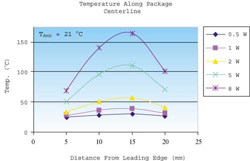 |
Figure 1. Temperature measured along the surface of a package centerline as a function of the distance from the front edge and power.
It is not uncommon to find data presented as in Figure 1. It shows the temperature at four locations on the top surface of a package, along the symmetrical centerline of the geometry, and, for this case, in a forced convection cooling environment. The data is useful as presented; however, just a little bit of experience reveals that the exact same data, presented in Figure 2, can be understood more completely. The presentation in Figure 2 is nothing more than the temperature rise recorded at each temperature location, divided by the power dissipated in the component.
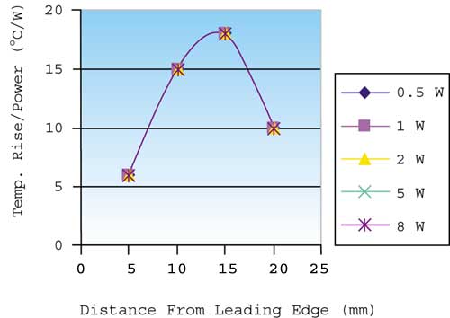 |
Figure 2. Data from figure 1 plotted as temperature rise over component power.
If the purpose of this data is to convey temperature rise information, Figure 1 performs this task very well. Imagine that a package designer would like to use this data to extrapolate how this component would perform at 10 W and consider which presentation of data is more useful. Clearly, Figure 2 is the better coordinate system for the extrapolation. Figure 2 shows that for the five power levels tested there is really only a single performance curve. This curve can be used to determine performance for a wide range of power levels, including a small amount of risky extrapolation.
This motivational example illustrates that combining variables can be very useful, but it does not do so by using dimensionless parameters. The sections that follow first describe the traditions and technique of combining variables into dimensionless groups, then go on to illustrate a few electronics cooling problems in dimensionless form.
Buckingham Pi Theorem
The Buckingham Pi Theorem states that a list of parameters used to describe a problem can be reduced in number by combining the variables using an algorithm that is based upon the dimensions of the variables. A complete statement of the theorem can be found in Kline, 1986. As is often the case, the complete statement of the theorem is more appropriate for individuals who are already comfortable with dimensional analysis than for people who are new to the topic.
A practical presentation of its application is pursued herein. Our goal is to learn to replace a list of variables, such as the four parameters associated with the data of Figure 1, with a shorter list. The tradition of dimensional analysis directs us toward a shortened list of parameters that are dimensionless and are referred to as groups.
For demonstration purposes we will use a problem that is important to the electronics packaging community: the pressure drop of a fluid as it moves through a duct with rough walls (Figure 3).
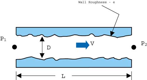 |
Figure 3. Flow through a pipe.
Based on experience, three of the important variables are combined immediately. The pressure drop
is divided by the length of pipe tested in order to obtain a pressure drop per unit length of pipe as a function of pipe diameter, wall roughness, mass density, dynamic viscosity and velocity. This is denoted functionally as
 |
This is a six variable problem. If we were to stay in the dimensional coordinate system implied by these variables we would end up performing much more testing than is required to evaluate the effects of each of the five independent variables on P/L. Instead we will reduce the number of parameters by organizing the six parameters into combinations that are dimensionless.
A dimensional analysis such as this can be expected to reduce the number of variables (via combination) by an amount up to a maximum that is equal to the number of primary dimensions in terms of which all of the variables are expressed. Working in the SI system the primary dimensions that are used to express each of the variables in Equation 2 are mass (M), length (L) and time (t). Note the force dimension (Newton) is not a primary dimension in the SI system. Whenever we encounter force we must replace 1 N with
 |
Because Equation 2 is expressed in terms of three dimensions we can expect that we will be able to reduce the number of variables by up to three. The goal is to reduce the six parameters to three non-dimensional groups. In order to accomplish this reduction we will choose three variables from the list of six and then try to determine how we might combine each of those three with the remaining three, one at a time, to form dimensionless groups. If we choose three variables such as D, p and V we can combine them with each of the remaining three as follows:
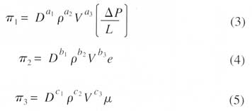 |
If the groups are to be dimensionless then we must determine what the exponents ai, bi, ci are in order for this to be so. The constants can be determined by using algebra similar to that shown in White, 1994. Referring to White’s Power Product Method, we write Equation 3 in terms of the dimensions of each of the parameters as
 |
1 is dimensionless hence its dimensions are shown as 1. The dimensions of each of the other parameters in Equation 3 are shown in terms of mass, length and time. The constants ai are now determined such that Equation 6 will have the same dimensions on both sides of the equal sign.
For the mass dimension to be the same on both sides we must have,
0=a2+1
For length, 0=a1-3a2 +a3
For time, 0=-a3 -2
Solving these expressions for ai yields:
a1 = 1 a2 = -1 a3 = -2
Substituting these exponents back into Equation 3 yields,
 |
Following a similar procedure to determine the exponents bi and ci we find,
 |
The results of this analysis process are three dimensionless variables where the pressure drop phenomena can be described as
The dimensionless pressure drop variable is only dependent upon two parameters. Rather than designing a test rig that can handle a variety of working fluids and a variety of surface roughness we can instead simply use a single fluid over a range of velocity and a pipe material with constant e and a range of pipe diameters.
Confession
The above example describes the six parameter pressure drop problem being replaced by a three parameter problem. Equation 7 states that the control of two parameters is enough to fix the third. While this discussion provides enough detail to allow the reader to perform some dimensional analysis it is important to point out that the logic presented herein does not prove that Equation 3 can be replaced by Equation 7. This proof is presented clearly and convincingly in White, 1994. Boyle, 1997 combines the work of White and others to provide a detailed presentation of the topic.
Examples
Electronics Characterization – RJa – Forced Convection
Figure 4 shows the geometric parameters that are important for the characterization of a single component on a board. A frequently encountered challenge is to characterize the thermal performance of this assembly in terms of the dependence of overall thermal resistance upon the following independent variables:
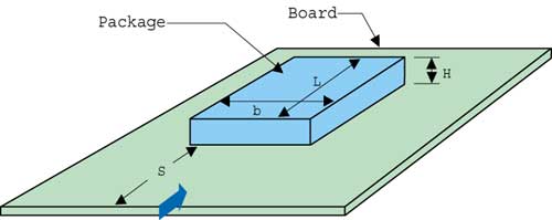 |
Figure 4. Geometry parameters for single component on a board.
 |
TJ – Junction (oC)
Ta – Cooling air (oC)
Q – Power (Watts) or ((kg m2)/s3)
S – Distance from leading edge of board (m)
b – Package width (m)
L – Length (m)
H – Height (m)
ka – Thermal conductivity of air ((kg m2)/s3)
kb – Board
kp – Package
p – Air density (kg/m3)
– Dynamic viscosity (kg/(m s)
V – Air velocity (m/s)
I – Turbulence intensity
Note that the analysis only includes the independent variables that the analyst considers important. This list is appropriate for a forced convection situation. Natural convection effects are included in the next example.
Equation 8 reveals a twelve parameter problem. All of the parameters in Equation 8 can be expressed in terms of mass, length, time and temperature. Therefore we can expect at best a reduction of four variables. If we choose to combine L, ka, V and pa with each of the remaining eight variables in turn, we find the following eight non-dimensional variables.
 |
This set of variables is still substantial but is much preferred to Equation 8. For a set of experiments performed either on a single model or for models of different scale but similar shape S/L, b/L and H/L are constant. Perhaps turbulence intensity is also constant or of secondary importance. Perhaps we are not changing the board material. Under these conditions the relationship that we must test to determine is:
 |
With this coordinate system we can report performance for a broad range of package types (kp), cooling air conditions, air velocity and even for various sized models and fit all of the results onto one graphical figure.
As a cautionary note, it must be stated that it is important to include all relevant independent parameters in order for these variables to be useful. For example, Equation 10 can not be used to characterize a problem where buoyancy effects are important, while buoyancy is included in the next example.
Electronics Characterization – RJa – Mixed Convection in a Vertical Duct
Figure 5 shows a test geometry where the effects of duct size, test model size and buoyancy on thermal resistance are evaluated. This problem could be investigated in the coordinates that are traditionally used by heat transfer specialists (Nusselt, Grashof, Prandtl).
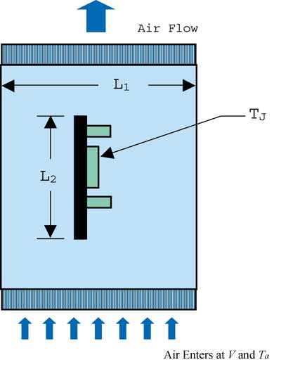 |
Figure 5. Vertical test duct for various sized models and ducts.
However, it is no less useful to work in terms of parameters that are closer to those familiar to the package designer. The list of variables that we will use is given in Equation 11.
In this case Q is included as an independent parameter in order to quantify the effect of buoyancy.
Each of the variables in the equation can be expressed in terms of the four dimensions mass, length, time and temperature. If we choose to combine L1,p, and ka with each of the remaining variables in turn we find a functional relationship between four non-dimensional parameters as follows:
 |
If experiments are performed at a constant Reynolds number, then by simply adjusting the size of the duct L1, and the power Q, characterizations can be obtained for a wide range of board size and fluid properties. Note that the buoyancy effect is managed by use of the variable (L1p2Q)/3. This variable is tied more closely to the traditions of electronics systems designers than the Grashof number that is used in the heat transfer literature.
Summary
The method of dimensional analysis and the Buckingham Pi Theorem provide an intuitive, convenient method of reducing the number of independent variables for most physical problems. By working in terms of a reduced number of non-dimensional parameters experiment designers and modelers are allowed significantly increased freedom for obtaining correlations for a range of applications. The method described herein can be used to find new coordinate systems for new problems. It is the author’s hope that the coordinate systems described in this article will find their way into use in industrial testing laboratories.
References
1. Boyle, M.T., Similitude in Electronics Cooling, a chapter in the text Thermal Measurements in Electronics Cooling, Edited by K. Azar CRC 1997.
2. Kline, S. J., Similitude and Approximation Theory, Springer-Verlag, Berlin, 1986.
3. White, F.M., Fluid Mechanics 3rd Edition, McGraw-Hill, New York, 1994.


