Introduction
The thermal design of today’s electronic equipment relies significantly on the use of Computational Fluid Dynamics (CFD) software for the prediction of electronics operational temperature. In the early to intermediate product design phase, CFD analysis is used to select a cooling strategy and refine a thermal design by parametric analysis. In the final design phase, detailed analysis of product thermal performance is performed to provide boundary conditions for performance and reliability prediction. However, it is recognized that progress in reliability prediction is currently hampered by the lack of methods to accurately predict electronics operational temperature, in terms of either absolute temperature, or spatial or temporal temperature gradients.
While over the last decade the pre- and post processing capabilities of CFD software dedicated to the thermal analysis of electronics have evolved considerably to improve the productivity of design analysis, their turbulent flow modeling capabilities have remained confined to zero-equation mixing length or standard two-equation high-Reynolds number k- eddy viscosity turbulence models. These models meet the criteria of robustness, in terms of promoting stable convergence, and to some extent, universality, which make them popular for practical engineering calculations. They are by far the most widely-used and validated, and are considered as computationally viable in a design environment. Unfortunately, this approach is not entirely satisfactory for modeling the thermal and kinematic complexity of thermofluid problems in forced air-cooled electronic systems. Based on experimental benchmarks, this article provides an overview of the potential shortcomings of the fluid flow modeling currently employed for populated Printed Circuit Board (PCB) thermal analysis, and illustrates the potential of alternative low-Reynolds number eddy viscosity turbulent flow modeling strategies to offer improved predictive accuracy.
Current Approaches to Turbulent Flow Modeling in Electronic Systems
The mixing length model and the high-Reynolds number k- model are considered as the industry-standard turbulent flow modeling approaches for electronics cooling. In the mixing length model the turbulent viscosity is expressed as a simple algebraic formula, based on the product of a turbulent velocity scale and length scale. Such models are intended for practical, coarse grid computations of global flow and temperature distributions, rather than for detailed component-board level analyses. The more sophisticated k-
turbulence model allows for the effects of transport of turbulence properties by convection and diffusion, and for the production and destruction of turbulence. Two partial differential transport equations, for the turbulent kinetic energy (k) and the rate of dissipation of turbulent kinetic energy (
), are solved.Both the mixing length and high-Reynolds number k-
models are primarily valid for turbulent core flows, and are not applicable in regions close to solid walls where viscous effects predominate over turbulent ones. To solve for the turbulent exchange of heat and momentum between solid surfaces and the fluid in the near-wall region, “law-of-the-wall” wall functions are employed. These are based on empirical formulae for wall surface friction and heat transfer, whereby heat and momentum flux are proportionalized through the Reynolds analogy. In this approach, the viscosity-affected inner region, comprising of the viscous sub-layer and buffer layer, is not resolved, but instead is bridged, with the wall functions generally requiring the near-wall fluid node to be located outside the viscous sub-layer. This approach eases the necessity for fine gridding in the near-wall region, which would otherwise be required to resolve it using an appropriate turbulence model.If turbulent fluid flow exists within electronic enclosures, it is usually confined and constrained by many closely spaced solid objects, which thus have the dominant effect in determining flow patterns, pressure drops and temperature distributions. To capture such flow fields, the use of the k-
model is generally required, but unfortunately for system level analysis its application is not feasible due to computationally excessive fine grid requirement, necessary to accurately represent the velocity gradients involved and hence estimate turbulent viscosity. Consequently, the mixing length models are typically employed for such analysis. However due to the dominant effect of near-wall turbulence on heat transfer, its representation may be more critical. In such instances the use of zero-equation models could provide reasonable estimates of turbulent viscosity, without introducing dramatic errors into heat transfer predictions, providing that the wall functions are applicable. This hypothesis forms the turbulence modeling strategy employed in CFD codes dedicated to the thermal analysis of electronics.Unfortunately, this strategy is not suited to the detailed analysis of heat transfer in air-cooled PCBs. Electronic systems contain complex geometries, numerous length scales, buoyancy forces and the fluid flow is often transitional with complex flow phenomena. Such phenomena are generated by cooling fans or intricate geometries, such as EMC screens, vents and populated circuit boards. Fan-generated flows contain swirling flow patterns, while screen holes will produce jets downstream. Such flow disturbances can generate unsteady or transitional flow conditions over electronic circuit boards, with attaching, separating and recirculating flow features. In addition, the component topology often generates multi-dimensional flow phenomena that include pulsating and vortical structures. Airflows over component-boards are usually classified as low-Reynolds number flows due to the small velocities and geometric length scales encountered, that contain pockets of turbulence generated by the component geometry. The standard k-
turbulence model is not specific for this type of flow. In addition, “law-of-the-wall” wall functions are justified for boundary layer type flows, but are inadequate for separating, reattaching or recirculating flow conditions where the Reynolds analogy does not hold. Furthermore, wall functions become less reliable in situations where low-Reynolds number or near-wall effects are pervasive in the flow domain.These limitations have been highlighted in two independent case studies that have assessed CFD predictive accuracy for PCB heat transfer [1,2]. Both studies showed that in forced convection conditions the operating temperature of all components could not be accurately predicted using either a laminar or standard high-Reynolds number k-
turbulent flow model, and concluded with the need for a flow model capable of modeling transition. Errors in predicted component junction temperature ranged from -10 to +22°C (up to 35%), with discrepancies of up to 10°C between flow models in aerodynamically sensitive regions. Prediction accuracy is anticipated to decay in real electronic systems, where more complex flow conditions and modeling uncertainties would both exist, with larger computational penalties.These difficulties are compounded by the fact that in an early design phase, the CFD user generally has little or no a priori knowledge of the flow regime over the board, whether laminar, transitional, turbulent, and steady or unsteady. Such an uncertainty arises from both the absence of a physical prototype for experimental characterization, and the difficulty in defining a characteristic dimension, hence transition Reynolds number, that adequately describes the heat transfer characteristic over the PCB. In spite of this difficulty, the onus is on the CFD user to select an appropriate flow modeling strategy.
In the above context, until improved flow modeling is employed, CFD predictions of PCB thermal performance should be interpreted with caution, both quantitatively and qualitatively. Ultimately, component operational temperature should be experimentally measured when used for strategic product design decisions and reliability predictions.
In the long term, however, the success of virtual prototyping methods will depend upon their accuracy. The authors therefore believe that a more robust thermal design methodology should aim at improved predictive accuracy rather than just enhanced design productivity. Such a change in philosophy would be required to enable critical product design decisions or reliability predictions to be made with confidence. This will require a change of focus from the electronics industry’s current demand for improved CFD code pre- and post-processing, towards improved flow modeling.
Alternative Strategies
Although a multitude of turbulence models has been developed, no universal model exists yet that performs superiorly and reliably for all classes of flows. In the absence of a universal model, the development of improved turbulence models specifically intended for distinct categories of flows is being actively pursued. Improved near-wall modeling can be achieved using turbulence models specific for low-Reynolds number, wall-bounded flows, which permit the governing equations to be integrated all the way to the wall, thereby eliminating the use of wall functions. Efforts in this area have focused on the development of two-equation models, which are typically considered as the minimum acceptable level of Reynolds stress closure.
Examples of two-equation models, available in general-purpose CFD codes, include low-Reynolds number variants of the k- and k-w models. Two-layer zonal model formulations are an alternative solution, whereby a one-equation (k) turbulence model is applied in the viscosity-affected near-wall region, and either a standard or more advanced k-
model is employed in the fully turbulent core region. In all above approaches the integration to the wall requires a very fine near-wall grid resolution in the viscous sub-layer, the application of which will be increasingly facilitated by computational advances and unstructured/embedded gridding technology.The potential of such turbulence modeling strategies to improve predictive accuracy for component operational temperature relative to the standard k-
model has been investigated using experimental benchmarks in [3]. A selection of these results is presented in the following case study for the Shear Stress Transport (SST) k-w model, as an illustrative example – the authors do not wish to advocate the use of this particular model over alternative candidate turbulence models. The SST k-w model blends a low-Reynolds number k-w model in the inner region of the boundary layer, and a high-Reynolds number k-
model in the outer part. It is generally considered to both be more robust and have a better degree of universality than either the low-Reynolds number k-
model or the standard k-w model.
Case Study
The test cases analyzed are based on the PCB shown in Figure 1, which is populated with fifteen thermally-enhanced 160-lead PQFPs. This PCB was thermally characterized in 2 and 4 m/s wind tunnel airflows. Two flow conditions were considered, namely with or without a controlled upstream flow disturbance. Test case complexity was incremented in controlled steps, from individually powered components to a simultaneously powered configuration, where all components are powered. This enabled the impact of both aerodynamic conditions and component thermal interaction on junction temperature prediction accuracy to be quantified. Benchmark criteria are based on component junction and component-board surface temperatures, measured using thermal test dies and infrared thermography respectively. The numerical models were built and solved using commercially available Finite Volume CFD codes, and are described in [2,3]. The component-board modeling methodologies have been previously validated [2,3].
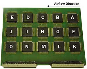 |
Figure 1. Multi-component test PCB. PCB size = 233 x 160 x 1.6 mm. The position of each component on the PCB is identified by the lettering, A to O. A, F and K are leading edge components.The results presented are confined to the central row components, F to J, Figure 1. The reader is referred to [2,3] for a detailed discussion on prediction errors in component operating temperature for both the laminar and k- flow models, and improved accuracy using the SST k-w model, with the salient findings summarized here.
|
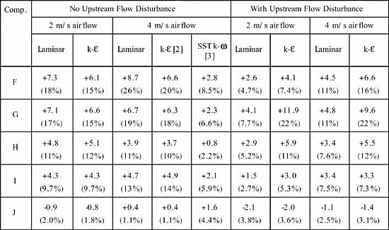
Individually Powered Components, Table 1
In the absence of upstream flow disturbance, the greatest prediction errors for both the laminar and k- flow models occur at the first two leading edge component rows, indicating a weakness to predict the leading edge flows, visualized in [2]. The SST k-w model displays improved predictive accuracy in this region, indicating improved prediction of leading edge flow.When flow disturbance is introduced upstream, the greatest prediction errors occur for component G using the k-
flow model, which is located in a region of strong flow re-attachment. The poor accuracy of the k-
model in this region is attributed to the limited applicability of the wall functions used for the prediction of wall shear stress, hence heat transfer in re-attaching flow conditions.
|
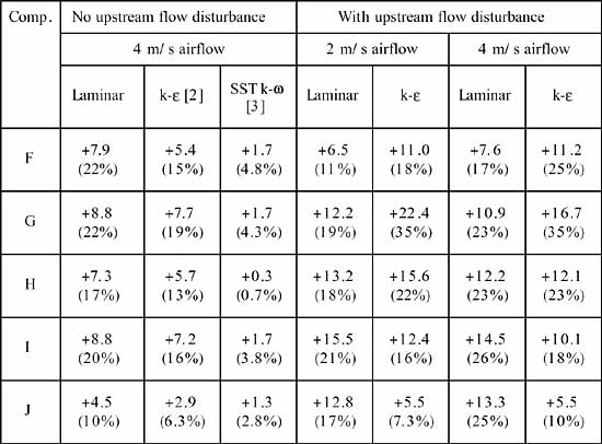
Simultaneously Powered Components, Table 2
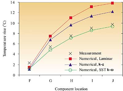
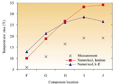
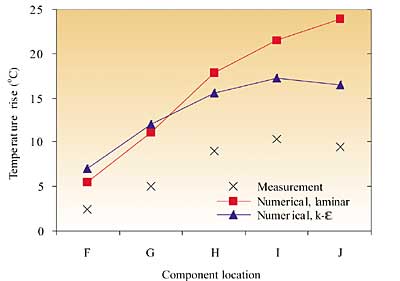
Using the laminar and k- models, prediction accuracy ranges from +3 to +22°C (up to 35%), with neither model yielding best accuracy for all components. These errors are attributed to inaccurate flow field prediction, impacting on the prediction of both aerodynamic conditions, as highlighted above, and component thermal interaction. The latter variable is analyzed in terms of the downstream component temperature rise between the individually- and simultaneously powered configurations in Figure 2. Whereas the laminar and k-
models overpredict this temperature rise by on order 40% and 25% respectively in Figure 2(a), the corresponding SST k-w predictions are within 4% of measurement. Such improvements are of significance, considering the combined trends of rising Integrated Circuit (IC) power dissipation and component packing density in electronic systems, which act to amplify component thermal interaction.
|
Conclusions
An overview of the potential shortcomings of the fluid flow modeling currently employed for populated PCB thermal analysis was presented. The potential of alternative low-Reynolds number eddy viscosity turbulent flow modeling strategies to improve predictive accuracy was illustrated. Such improvements would enable parametric analysis of product thermal performance to be undertaken with greater confidence, and could contribute to the generation of more accurate temperature boundary conditions for use in reliability prediction.
Vendors of CFD codes dedicated to the thermal analysis of electronic equipment should consider the adoption of turbulence models more suited to detailed board level analysis. Further benchmarks are required to identify candidate turbulence models capable of performing well for a wide range of PCB applications.
References
- Rodgers, P., Eveloy, V., Davies, M.R.D., “An Experimental Assessment of Numerical Predictive Accuracy for Electronic Component Heat Transfer in Forced Convection: Parts I and II,” Transactions of the ASME, Journal of Electronic Packaging, Vol. 125, No. 1, 2003, pp. 67-83.
- Eveloy, V., Rodgers, P., Hashmi, M.S.J., “Numerical Prediction of Electronic Component Operational Temperature: A Perspective,” IEEE Transactions on Components and Packaging Technologies (in press), 2004.
- Eveloy, V., Rodgers, P., Hashmi, M.S.J., “An Experimental Assessment of Computational Fluid Dynamics Predictive Accuracy for the Prediction of Electronic Component Operational Temperature,” Proceedings of the ASME Summer Heat Transfer Conference, HT2003-47282, 2003.

