Design of Experiments for Numerical Parameter Studies of Electronic Systems: Optimizing the Cooling Strategy of an Ethernet Switch

Introduction

As electronic products become more sophisticated and design margins tighten, defining the thermal management strategy early in the design cycle is vital to ensure a cost-effective design for the level of heat dissipation. Optimizing the cooling system for an electronic product can involve juggling many design parameters, such as airflow rate, fan and vent locations, and heat sink size.

Numerical tools are increasingly used in the physical design of electronic products to qualify and improve the design and reduce time to market. However, despite the computing power available, exploring all possible design alternatives is extremely time-consuming. Usually in such a situation, thermal engineers use their intuition and experience, carry out a number of simulation runs, and choose the best design. In this process, the engineers can benefit considerably from techniques and tools from “Design of Experiments” and “Mathematical Optimization”, especially in case of multi-disciplinary design challenges.

This article presents an efficient approach for doing parameter studies and optimizing numerical models. The approach elaborates and extends on both “Response Surface Modelling” [1] and “Design and Analysis of Computer Experiments” [2], and consists of three steps:

1. Design of Computer Experiments (DoCE) – Definition of design parameter space, generation of a set of suitably chosen designs, and numerical simulation of these designs.
2. Response Surface Modelling (RSM) – Construction of response surfaces for all relevant quantities calculated by the analysis tool. Examples: junction temperatures, pressure drops, and fan flow rates. Validation of these response surfaces.
3. Mathematical Optimization – Optimization of response surfaces. Validation of optimum design by simulation.

 

These steps will be illustrated in this article by considering the redesign of an existing Ethernet switch. Redesign is necessary because of a new board design that does not meet the cooling requirements of the board components. For this we used a general-purpose design optimization tool [3] in conjunction with a state-of-the-art CFD-code [4]. Please consult [5,6] for a more in-depth discussion.

Ethernet Switch

Consider an existing Ethernet switch that does not meet the cooling requirements of the components because of a new board design. The current switch box (127 x 178 x 44 mm) with the new board layout is shown in Figure 1. The current configuration draws air in through one vent opposite a fan on the other end of the box. The five major components are labelled C1�C5.

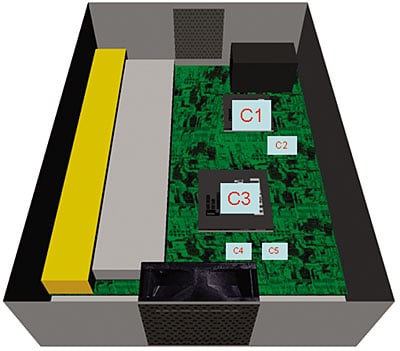Figure 1. Current switch box with new board layout.The thermal behaviour of the system is calculated using the CFD code. The results based on a 35°C ambient showed that component C2 is operating above its maximum junction limit. The task at hand is to determine if the current venting and fan configuration can be sufficiently enhanced to meet the cooling requirements of C2 as well as maximize the operating margin for the other components.

Table 1. Results First Scenario

Component Tj-limit (°C) Tj (°C) Margin (%) C1 125 112 16 C2 125 110 20 C3 125 121 5 C4 100 80 45 C5 100 80 45

The first scenario considered was created in an ad hoc fashion with a 35 x 100 mm vent placed on the wall opposite the ports as shown in Figure 1. Table 1 shows the simulated junction temperature and the operating margin for the five major components for a 35°C ambient, where operating margin is given by:

After adding this vent none of the major components operates above its junction limit. However, component C3 has only a small operating margin. The remainder of this article focuses on optimizing the venting and fan configuration in order to maximize the operating margin for all components. The results will support the designer in deciding if an additional vent is a viable cooling alternative as a function of its size and location.

Design of Computer Experiments

The art of efficiently setting up experiments is called Design of Experiments (DoE) [7]. Classical examples of DoE techniques are full factorial, Box-Behnken, Taguchi, and Central Composite. Designing computer experiments differs from classical DoE, which typically considers physical experimentation. Virtual experimentation is not subject to the noise or uncertainty associated with physical measurements. An appropriate design of computer experiment should be:

• Space Filling – Due to the noise associated with physical experimentation, classical DoE would focus on parameter settings near the perimeter of the design region. Computer simulation is not subject to this constraint. A space filling scheme distributes the design parameters equally throughout the design space.
• Non-Collapsing – Due to the absence of noise in numerical experimentation it is not beneficial to conduct more than one experiment with the same design parameter settings. A simulation scheme is called non-collapsing if, in case one or more of the design parameters appear unimportant, every point in the scheme still gives information about the influence of the other design parameters on the response.

 

We propagate the use of space-filling Latin Hypercube Designs (LHD) [8], ensuring that the design parameters are equally spaced throughout the design region and every experiment will be unique. In [2] the space-filling LHD was extended to deal with general design constraints, which are important in optimizing cooling strategies [9].

To optimize the operating margins for all major components of the Ethernet switch, a parameter study is set up. The additional vent is allowed to vary in size and position as indicated in Table 2. The fan location was allowed to vary laterally from its original location to a maximum displacement of 70 mm. Table 2 summarizes all design parameter and their ranges. To ensure that the vent will not extend the past edge of the enclosure (150 mm), a linear design constraint was added.

Table 2. Design Parameters and Bounds

Design Parameter Unit Minimum Maximum Fan       Y location mm 0 70 Side Vent       Z size mm 10 35 X location mm 15 150 X size mm 15 100

The optimization tool was used to create a space-filling LHD of 20 designs within the design space. Figure 2 plots for each design the smallest operating margin of any of the major components. As a result of this first design space exploration, a design was found for which the operating margin for all components is larger than or equal to 24%.

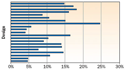Figure 2. Smallest operating margin.

Response Surface Models

In recent years a lot of work has been done in the area of modeling of output of computer simulation models; see for instance [1]. The two most popular model types are simple linear or quadratic regression models and Kriging models. In general, the latter models yield the best approximations when the underlying relationship is highly non-linear.

When using approximations of computer simulation models, validation is very important. Response surfaces are usually validated by calculating some validation statistic of the differences between simulated and predicted values. An example of such a statistic is the Root Mean Squared Error (RMSE) function. Often such validation statistics are calculated on the same data set as was used to build the compact model. The lower the mean squared error, the better the model mimics the data. This leads to the disadvantage that it does not account for the effect of over-fitting: by making the compact model arbitrarily complex, the function value can be made arbitrarily small. In the extreme case of interpolating compact models (e.g., Kriging models) the value of such a cost function can easily be made equal to zero. It is not the mimic capabilities but the prediction capabilities of a model that should be assessed. Therefore we propagate the use of one of the following techniques for validating the prediction capabilities of a compact model.

• Independent Test Set – Assess the prediction capabilities of the compact model on an independent test set and calculate the desired validation statistics. A major disadvantage is that extra, often time-consuming, simulations must be performed.
• Cross-Validation – Re-estimate the compact model n times, with n equal to the number of data points, while each time skipping one of the data points. Every time, the skipped data point is used to test the prediction capabilities by calculating the desired statistic. In this article we will use the cross-validation RMSE (CV-RMSE) for validation purposes.

 

The optimization tool was also used to build responses surfaces that describe the relationship between vent/fan parameters and operating margins (OM1,..,OM5) and temperatures (T1,�,T5). Using a stepwise procedure based on cross-validation, quadratic models were obtained.

Figure 3 shows a plot of T2 against the “x” location of the side vent for four different values of the “y” location of the fan.

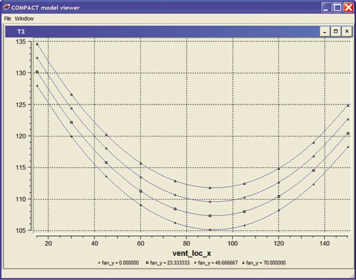Figure 3. Temperature T2 as function of fan and vent location.Table 3 shows the validation results for the constructed response surfaces. Looking at the CV-RMSE values, we conclude that the absolute difference between predicted and simulated temperatures is 1-3°C on average. For the operating margins this difference is 2-4%. For our purposes this is sufficiently accurate. Note that the ordinary RMSE value is too optimistic.

Table 3. Validation Results for Response Surface Models

RSM R2 R2adj RMSE CV-RMSE T1 1.00 0.99 0.35 0.76 T2 0.91 0.86 1.46 2.42 T3 0.97 0.94 0.79 1.49 T4 0.96 0.93 0.52 0.86 T5 0.97 0.95 0.42 0.72 OM1 0.99 0.99 0.71 1.55 OM2 0.92 0.87 2.19 3.53 OM3 0.97 0.95 1.08 2.08 OM4 0.96 0.93 2.27 3.61 OM5 0.97 0.94 1.96 3.48

Optimization of Response Surfaces

Design optimization consists of finding values for the design parameters that satisfy all constraints and minimize some chosen objective function. The validated response surface models are usually optimized using techniques from Mathematical Programming, like Non-Linear Programming (NLP). The possible existence of local minima makes it necessary to apply a global optimization strategy. The optimization tool uses a multi-start approach, meaning that several local optimizations are started sequentially.

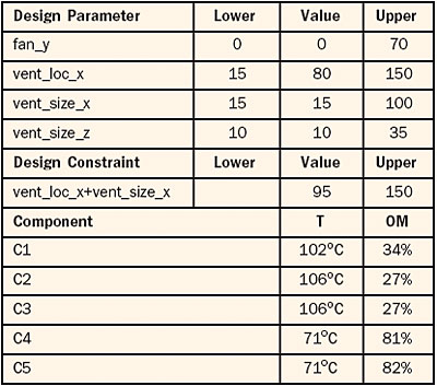
In the Ethernet case the problem is to choose the venting and fan configuration so that all design constraints are satisfied and the minimal operating margin is as large as possible. First we investigate optimal cooling strategies for individual components. Table 4 shows the optimal venting and fan configuration when, respectively, the operating margin for C1, C2, � is maximized. It appears that components C2 and C3 have a similar optimal cooling strategy. The same holds for components C4 and C5. Component C3 is the bottleneck with a maximal OM of 29%. Optimal cooling configurations for the three most critical components C1, C2, and C3 are equal except for the value of the “x” location of the side vent (vent_loc_x). In favour of the most critical components, vent_loc_x was set to 80 mm.

Table 4. Optimal Cooling Configuration for Major Components

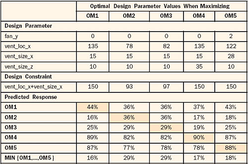The final step is to verify this optimum cooling configuration using the CFD code. Table 5 shows that the minimal simulated operating margin is 27%.

Table 5. Validation Run for Optimum Cooling Configuration

Summary and Conclusion

The differences between the ‘classical’ Design of Experiments (DoE) and Design of Numerical Experiments have been highlighted. ‘Classical’ approaches, such as the popular Taguchi schemes, are not the preferred choice when experimental noise is absent. For numerical ‘experiments’ the use of Latin Hypercube Designs is recommended. The method has been illustrated by optimizing the thermal behaviour of an Ethernet switch by varying the fan location and the vent size/location. The focus is on the so-called operating margin, which is essentially a measure of how close the component temperature is to the maximum allowable temperature. The results show clearly the benefits of the proposed approach. The best design offered a smaller vent while increasing the minimal operating margin from 5% to 27%. In the optimum design described in this article, three parameters were set on the minimum value allowed in the experiments. Hence, it is likely that even further margin could be gained by enlarging the design space.

Acknowledgement 

The author appreciates the support of John Wilson from Flomerics for providing the case and data.

References

1. Myers, R.H., “Response Surface Methodology – Current Status and Future Directions”, Journal of Quality Technology, No. 31, 1999, pp. 30-74.
2. Sachs, J., Welch, W.J., Mitchel, T.J., and Wynn, H.P., “Design and Analysis of Computer Experiments”, Statistical Science, No. 4, 1989, pp. 409-435.
3. COMPACT, www.cqm.nl/pages002/structure/section003/009/page004/index.asp
4. FLOTHERM, www.flomerics.com
5. Stehouwer, H.P. and Hertog, D. den, “Simulation-Based Design Optimization: Methodology and Applications”, Proceedings of the First ASMO UK / ISSMO Conference on Engineering Design Optimization, Ilkley, UK, 1999.
6. Hertog, D. den and Stehouwer, H.P., “Optimizing Color Picture Tubes by High-Cost Nonlinear Programming”, European Journal on Operational Research, No. 140, 2000, pp. 197-211.
7. Montgomery, D.C., Design and Analysis of Experiments, John Wiley & Sons, New York, 1984.
8. Morris, M.D. and Mitchell, T.J., “Exploratory Designs for Computer Experiments”, Journal of Statistical Planning and Inference, No. 43, 1995, pp. 381-402.
9. Parry, J., Bornoff, R., Stehouwer, H.P., Driessen L.T., and Stinstra, E.D., “Simulation-Based Design Optimization Methodologies Applied to CFD”, Proceedings SEMITHERM XIX, San Jose, 2003, pp. 8-13.