Today virtually all serious thermal analysis and design calculations for electronic packages are performed using various commercial flow and thermal conduction codes. Nonetheless, there are still many instances, especially in the early phases of a project, when the thermal engineer finds it advantageous to perform so called “back of the envelope” calculations without resorting to such codes. For example the calculation may be as simple as using a two element series resistance model to determine the relative merit of improving either the internal or external thermal resistance of a circuit module.
 |
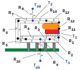
Figure 1. Example of a thermal resistance network for a single chip module with a thermal grease pad between chip and cap.
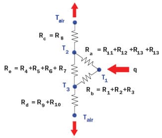
Beyond this a more detailed model may be created to obtain a preliminary estimate of overall thermal resistance from chip to cooling fluid considering multiple thermal resistances and heat flow paths. As long as the model is comprised only of parallel and series thermal resistances it is readily reducible to a single overall or equivalent thermal resistance. However, this is sometimes not the case, as in the example shown in Figure 1. In this example a layer of thermal paste is used to provide an alternative heat flow path bridging the gap from the chip to the package cap. In Figure 2, the resistances from Figure 1 that are in series have been added together to form resistances Ra, Rb, Re and Rd. Without the thermal paste layer, the thermal resistance across the gap, R12, is so large as to effectively make Ra infinite taking it out of the picture as a heat flow path and thereby reducing the thermal resistance network to a series-parallel combination of resistances. With the thermal paste layer in place, the magnitude of R12 is substantially reduced so that the heat flow path through Ra cannot be ignored. It should be evident by inspection of Figure 2, that in this latter case the thermal network cannot be further reduced as a series-parallel combination of resistances. Those readers who recall their DC circuits course may recognize that in this particular case a Y-Δ transformation could be used to convert the resistance network into a series-parallel combination. However, this will not be done here, as the object of this article is to illustrate how a matrix algebra method may be used to solve for the overall thermal resistance.
 |
Figure 2. Simplified thermal resistance network representing module shown in Figure 1.
Using a matrix algebra method it is possible to calculate the temperature at each node for a given chip heat load and then the total thermal resistance from chip junction to air. To do this it is first necessary to write a heat balance equation for each temperature node. The heat balance equation is simply an algebraic statement that under steady-state conditions the heat flowing into a node is equal to the heat flowing out of the node. Although, we generally think in terms of thermal resistances, it will be more convenient here to write the necessary heat balance equations in the form of thermal conductances. The heat flow from one node to another node is given by
where thermal conductance, K, is simply the reciprocal of thermal resistance, R, and ΔT is the temperature difference between the nodes.
For node T1, which represents the temperature on the device side of the chip, the heat balance equation is,
q = Ka × (T1 – T2 ) + Kb × (T1 – T3 ) (2)
where q is the chip heat load and Ka and Kb are the thermal conductances associated with thermal resistances Ra and Rb. In other words, equation (2) is an algebraic way of stating that the heat dissipated by the chip and entering node T1 is equal to the sum of the heat leaving node T1 and flowing through thermal conductances Ka and Kb to nodes T2 and T3 respectively. This statement is analogous to Kirchoff’s Current Law which states that the sum of currents into a junction is equal to the sum of currents out of the junction. The next step is to rearrange equation (2) so that the thermal conductances are grouped together multiplying unknown temperature variables T1, T2 and T3 respectively on one side of the equals sign and the known constant term, q, is placed on the other side of the equals sign as follows,
(Ka + K b ) × T1 – K a × T2 – K b × T3 = q (2a)
In a similar fashion the heat balance equation for node 2 may be written as,
Ka × (T1 – T2 ) + K e × (T3 – T2 ) = K c × (T2 – Tair ) (3)
and again after rearranging, equation (3) becomes
−Ka × T1 + (K a + K e + K c ) × T2 – K e × T3 = K c × Tair (3a)
In this instance, the constant term on the right-hand side of equation (3a) is the product of thermal conductance Kc and the temperature, Tair, of the cooling air.
Finally for node 3, the heat balance equation is
K b × (T1 – T3 ) = K d × (T3 – Tair ) + K e × (T3 – T2 ) (4)
and after rearranging (4) we obtain
– K b × T1 – K e ×T2 + (K b + K d + K e )×T3 = K d ×Tair (4a)
with the product of thermal conductance Kd and air temperature, Tair, as the constant term on the right-hand side of equation (4a).
Now for the matrix part of the method. For those readers who have studied linear algebra and matrices, you may skip this paragraph and go to the next one. For those who are unfamiliar with matrices or remember a matrix algebra course in the past with some degree of displeasure, please do not abandon me now but keep reading. For the matter at hand, all that you really need to know is that matrices are a mathematical way of representing simultaneous linear algebra equations in a compact fashion! Equations (2a), (3a) and (4a) are simply a set of simultaneous linear algebra equations that can be expressed as
K11T1 + K12T2 + K13T3 = b1 (5a)
K21T1 + K22T2 + K23T3 = b2 (5b)
K31T1 + K32T2 + K33T3 = b3 (5c)
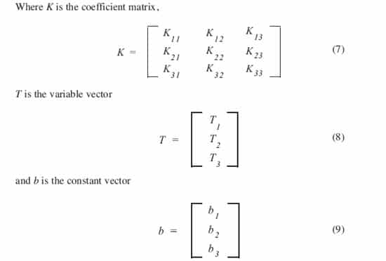
Where the coefficients K11, K12 . . . . K33, are the signed combinations of thermal conductance terms multiplying temperature variables T1, T2, and T3 on the left-side of equations (2a), (2b) and (2c) and constants b1 , b2 , and b3 are the constant terms on the right-side of the equations. In matrix notation these same equations can be compactly represented as
K • T = b (6)
 |
Now to solve a matrix equation such as (6) for the temperature variable T, all we need to do is multiply the constant vector b by the matrix inverse, K-1, of the coefficient matrix K,
K-1 • b = T (10)
Of course the obvious question a reader may ask is — “How do I calculate the inverse matrix K-1 “? The curt answer might be — “If I have to tell you, you won’t want to bother”. Fortunately, you don’t have to calculate it on your own. Many computational aids such as MathCAD [1], Matlab [2] and EXCEL [3] and others can be used to obtain the matrix inverse of the coefficient matrix and multiply it times the constant vector to obtain the desired solution vector.
Now returning to our example problem, the rearranged heat balance equations (2a), (3a) and (4a) can be expressed in matrix form as
 |
and the solution for the temperature at each of the nodes may be expressed in matrix form as
 |
Table 1. Values of Individual Thermal Resistances.
|
Table 2. Values of Thermal Resistance and Corresponding Thermal Conductance
|
To provide a numerical illustration of the solution, the example values of thermal resistance given in Table 1 for each part of the thermal paths were used. Individual thermal resistances were combined as shown in Figure 2 to calculate thermal resistances Ra, Rb, Rc, Rd and Re, and their corresponding thermal conductances Ka, Kb, Kc, Kd and Ke. The values obtained are shown in Table 2 and were used in equation (12) to obtain the numerical values in equation (13)
 |
and multiplying the constant vector by the inverse of the coefficient matrix we obtain the temperature at each of the three nodes:
 |
A chip heat load of 1 watt and an air temperature of 25 °C were used to obtain the results shown in equation (14). These values may now be along used with the chip temperature, T1, obtained above to determine the total package thermal resistance to air,
Although the problem presented here as an example, only involved the solution of three simultaneous equations, the same method can be readily extended to more involved thermal networks resulting in many more simultaneous equations. As such it is powerful tool for conducting preliminary thermal calculations before turning to commercial codes for detailed thermal analyses.
References


