Introduction
In today’s demanding business climate, thermal engineers are often called upon to produce thermal analyses rapidly. For example, there is frequently the need for a quick calculation of a JEDEC-standard thermal performance metric, such as ΘJA (junction-to-ambient thermal resistance), for specific IC package designs on the basis of limited data. These metrics are in the wide use in the electronics industry[1].
Very often there is neither the time nor sufficient information regarding the internal construction of a package or its constituent materials to perform a detailed finite element simulation.
It can be very expedient to be able to use existing test data for a family of packages to generate correlations to predict the thermal performance of a particular package from that family.
Conventional methods of doing this involve the creation of structured data sets, such as those prescribed by Design of Experiments (DOE) methods. While this is certainly possible in principle, the thermal engineer most often finds himself in the position of “mining” the available data.
At the most basic level, the analysis of the thermal performance of a family of packages can take the form of a graph of ΘJA versus the body size of each of the packages. The end result usually can be represented by a trend line, which is a smooth, monotonically decreasing function. This sort of behavior can usually be captured reasonably well by fitting a power law of the form Y(x) = bxm to the data. This sort of power law behavior is also frequently observed if one fixes the body size and then varies the size of an internal component of the package, such as the die.
This article describes a method involving a multi-parameter, power-law regression fit that can be useful in generating correlating ΘJA values to package design parameters. It is assumed here that the various packages in a family represent a reasonably consistent design approach.
Examples of parameters are [2,3]:
- Source width representing different length scales: package width and die width and, in a leadframe package, pad width.
- Parameters affecting spreading conductance in package such as the aggregate copper thickness in a Plastic Ball Grid Array (PBGA) substrate or the product of the leadframe thickness and thermal conductivity in a leadframe package.
- Thermal conductivity of material transmitting heat from die to nearby portions of package: die attach, molding compound.
Calculation Method
The following method, as applied to both a single- and multi-parameter analysis, is described below. While it has not been developed on the basis of mathematical rigor, it has proven consistently useful in practice in performing analyses of the sort in question.
Power-law Regression Fit for a Single Parameter
This method is performed using the following operations:
- Create table in spreadsheet
- Column #1 for parameter, p
- Column #2 for associated value of ΘJA
- One row for each package configuration being analyzed
- Calculate log, base 10, for each value
- Perform single-parameter linear regression
- log(ΘJA) = m* log(p) + b
- where m = slope, b = y intercept
- Take the anti-log of each side of the equation
- 10log(ΘJA) = 10m*log(p) + b
- ΘJA = 10b*p
Power-law Regression Fit for a Multiple Parameters
The preceding method can be extended to the analysis of n parameters as follows:
- Create table in spreadsheet
- Column #1 through #n, for parameter p1 through pn
- Column #n+1 for associated value of ΘJA
- One row for each package configuration being analyzed
- Calculate log, base 10, for each value
- Perform multi-parameter linear regression
- Process output values m1 through mn and b in a manner analogous to single parameter case
- Result: ΘJA = 10b * p1m1 * p2m2 * …. * pnmn
Determine Statistical Significance of Each Parameter
The statistical significance of each parameter can be estimated by the use of the following procedure to calculate the significance value (as defined herein).
- Calculate the significance value for each parameter:
- Rank parameters according to the calculated values of the significance value
- Perform regression starting with a single parameter having the largest significance value. Calculate root mean squared (RMS) error using the measured and predicted values of ΘJA, for all packages in the sample population, with a total of M samples
- Sequentially repeat the regression, adding the parameter with the next largest significance value
- With each new iteration apply test:
- Trend should have physical significance
- RMS error should be less than that of previous iteration
- If the test fails for a particular parameter, exclude it from the analysis.
Example — Quad Flat Package (QFP)
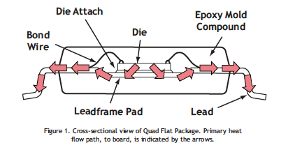
The methods described above are illustrated using a popular leadframe package format, the QFP. The internal construction of a standard QFP is illustrated in Figure 1. It also depicts the main path for the heat to flow from the chip to the attached board.
Table 1 lists the package parameters evaluated. They are nine in number and are all associated with this primary heat flow path. A total of 24 packages were represented in this analysis.
Table 1. Parameter Significance Analysis
| Parameter Index | Parameter | Min Value | Max Value | Units | mi | Significance Value | Physical Trend? |
|---|---|---|---|---|---|---|---|
| 1 | Body Size | 7 | 40 | mm | -0.390 | -0.231 | Yes |
| 2 | Pad Size | 5 | 16 | mm | -0.511 | -0.197 | Yes |
| 3 | Lead Count | 32 | 304 | N/A | 0.112 | 0.421 | No |
| 4 | Inner Lead-Pad Separation | 0.3 | 1.3 | mm | 0.049 | 0.071 | Yes |
| 5 | Body Thickness | 1.01 | 3.8 | mm | 0.029 | 0.039 | No |
| 6 | Die Size | 3.8 | 10.16 | mm | 0.144 | 0.184 | No |
| 7 | LF Thick * Th Cond | 25.5 | 38.227 | mm*W/mK | -0.040 | -0.014 | Yes |
| 8 | EMC Th Cond | 0.67 | 0.83 | W/mK | 0.346 | 0.067 | No |
| 9 | D/A Th Cond | 0.56 | 2.5 | W/mK | 0.143 | 0.219 | No |
Table 2. Sample Spreadsheet – 2-Parameter Analysis
| COLUMN | A | B | C |
| ROW | |||
| 1 | Body Size Avg (mm) | Pad Size (mm) | Th,ja (°C/W) |
| 2 | 7 | 5 | 47.9 |
| 3 | 10 | 6 | 41.1 |
| 4 | 10 | 7.4 | 37.5 |
| 5 – 16 | “ | “ | “ |
| 17 | 40 | 14.0 | 23.6 |
| 18 | |||
| Rows 19 – 36 showing embedded formulas | |||
| 19 | =LOG(A2) | =LOG(B2) | =LOG(C2) |
| 20 | =LOG(A3) | =LOG(B3) | =LOG(C3) |
| 21 | =LOG(A4) | =LOG(B4) | =LOG(C4) |
| 22 – 33 | “ | “ | “ |
| 34 | =LOG(A17) | =LOG(B17) | =LOG(C17) |
| 35 | m2 | m1 | b |
| 36 | {=LINEST(C19:C34,A 19:B34,TRUE,FALSE)} | {=LINEST(C19:C34,A 19:B34,TRUE,FALSE)} | {=LINEST(C19:C34,A 19:B34,TRUE,FALSE)} |
| Rows 19 – 36 showing calculated values | |||
| 19 | 0.845 | 0.699 | 1.680 |
| 20 | 1.000 | 0.778 | 1.614 |
| 21 | 1.000 | 0.869 | 1.574 |
| 22 – 33 | “ | “ | “ |
| 34 | 1.602 | 1.146 | 1.373 |
| 35 | m2 | m1 | b |
| 36 | -0.6614 | -0.0673 | 2.2021 |
The calculated values of the significance value are presented. For all of the parameters with the exception of the inner lead-pad separation, ΘJA is expected to decrease as the parameter is increased. Hence, for these parameters, a negative significance value would be consistent with the expected physical behavior. However, the following five parameters had a positive significance value: lead count, body thickness, die size, epoxy molding compound and die attach thermal conductivity. Hence, they were eliminated from further consideration.
The remaining parameters are highlighted in yellow in the table. Of these, the inner lead-pad separation and leadframe thickness * thermal conductivity had a significance value much less than the body size and pad size. Hence, the only parameters included in the subsequent analysis are the body size and pad size.
Results Calculation and Error Analysis
In order to perform a basic statistical test of the accuracy of this method, the population of 24 packages was separated by random selection into a training set, consisting of 16 packages, and a test set, consisting of the remaining eight.
Table 2 depicts the structure of an Excel® spreadsheet for 40 performing a 2-parameter analysis of the training using body size and pad size as independent variables.
Note that the formulas in the cells, A36, B26, and C36 represent an array. Please see the spreadsheet help menu for instructions on how to create the array after inputting the formula in cell A36. The regression coefficients are displayed in these same cells. Note that the input portion of the spreadsheet sequences the parameter columns from left to right, but Excel generates the mi coefficients from right to left.
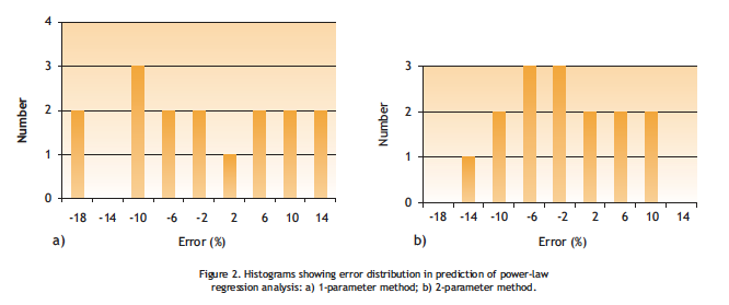
Figure 2 displays histograms for 1-parameter and 2-parameter fits to the training set. The 1-parameter fit is characterized by error values ranging from -20% to + 20% and an RMS error of 11%. In contrast, the 2-parameter fit manifests significantly smaller error values: max/min error range = ± 14% and RMS error = 7%.
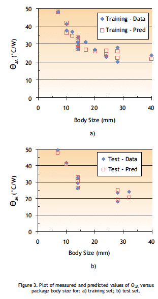
Figure 3 provides a comparison of the original data and predicted values for a) the training set and b) the test set. A qualitative comparison of the two graphs suggests that the method provides comparable accuracy for each set. This is confirmed by a calculation of the RMS error: training set, 7%; test set, 8%.
These results suggest that this method has a measure of robustness and that its predictive abilities, in this case, are not dependent upon some fortuitous selection of input data and package parameters.
Discussion
The ultimate success of this method in extracting the relationship between the thermal metric in question and a particular package parameter depends on the vagaries of the data set available to the thermal engineer. Hence, there is no guarantee that this method will be successful in extracting correlations between the thermal metric and a given parameter. However, as practiced by this author, it has proven useful in numerous instances in generating most of the correlations of interest. In general, it will be more successful with packages having a high level of heat spreading, whose thermal performance is usually less sensitive to variations in particular design details. It should be noted that, in the interest of putting these results into perspective, the QFP is not one of those packages.
The fact that the functional relationship between the thermal metric is a power law, rather than a higher order polynomial as is typical of DOE methods, has the consequence that there are no inflections in the derived correlations. This makes them reasonably robust and, within limits, able to make useful predictions for values of the parameters beyond the input range.
Conclusions
A relatively simple analytical procedure was developed for obtaining correlations between a thermal metric and statistically significant package parameters in a non-structured data set. This method was demonstrated to provide an RMS error in the range of 7-8% for a family of QFPs, when a 2-parameter analysis was employed. This method has been successful, in the past, in generating useful correlations involving a larger number of parameters for packages with an internal structure providing enhanced heat spreading.
References
- Guenin, B., “Component Thermal Characterization,” ElectronicsCooling, Vol.7, No.1, February, 2001.
- Guenin, B., “Packaging: Designing for Thermal Performance,” ElectronicsCooling, Vol.3, No.2, May, 1997.
- Guenin, B., “The Many Flavors of Ball Grid Array Packages,” ElectronicsCooling, Vol.8, No.1, February, 2002.


