Ross Wilcoxon
Rockwell Collins
Cedar Rapids, Iowa
A thermal resistance network analysis begins by defining discrete points within a system, known as nodes, and the thermal resistance between each set of nodes. Boundary conditions for external heat inputs and reference temperature(s) are applied to the appropriate nodes. Equations to relate nodal temperatures can be generated by applying an energy balance on each node in the system. This is identical to the approach used in electrical engineering to determine voltages at each point in an electrical resistance network.
One significant limitation of the thermal resistance analysis, as compared to the electrical analysis, is that there is much less difference in conductivity between thermal insulators and conductors (~4 orders of magnitude) than in their electrical counterparts (~20 orders of magnitude) [1]. Therefore, the analyst using a thermal resistance network needs to recognize that there are no perfect thermal insulators and all the nodes in a network are connected to some extent. While this can limit the precision of the approach, thermal resistance analysis can be an effective tool for understanding general behavior of a system and identifying those design factors that are most critical. This is especially true early in the design of a new system when limited knowledge of specific geometric parameters may limit the analyst’s ability to create a meaningful finite element model. One may think of resistance network analysis as one method for bridging the gap between ‘back of the envelope’ calculations and high level finite element analysis using dedicated analysis software.
A matrix analysis is a very effective method for solving nodal temperatures in a resistance network. The mechanisms for applying the matrix method have been presented in numerous publications, including [2]. Therefore the complete mathematical derivations will not be repeated here. As indicated in [2], mathematical software packages such as MathCAD or Matlab are ideal for solving matrix equations. However, many practicing engineers do not use these programs on a regular basis (if they even have access to them) and learning the software may take more time than solving the actual problem. Moreover, if the matrix solution software is not widely used within a company, it may be difficult to share the calculation tool with colleagues.
On the other hand, the majority of engineers use a spreadsheet, such as Microsoft Excel, on a regular basis. While it is recognized that spreadsheets aren’t as efficient for solving these types of problems as dedicated mathematical software, their ubiquity of use by engineers does make them very easy to share with others and to integrate the solutions into other spreadsheet based tools. This article will describe a step-by-step process for defining a thermal resistance network in Excel and using standard functions to solve for nodal temperatures in steady state heat transfer.
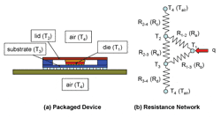
To illustrate the basic approach for using Excel to solve a thermal resistance network, the same problem outlined in [2] will be used. In that problem, a number of individual resistance terms were included in assessing the overall thermal characteristics of an integrated circuit package attached to a circuit board. A representation of the packaged device and the resulting simplified resistance network are shown in Figure 1. This network includes four nodes: Node 1 is the silicon die, Node 2 is the top of the package, Node 3 is the package substrate and Node 4 is the surrounding air. The resistances between the nodes are generally combinations of multiple series resistances.
In this article, the nomenclature used for each resistance indicates which two nodes it connects (i.e., R2-3 represents the total thermal resistance between Node 2 and Node 3). This nomenclature differs from that used in Ref. [2]; the symbols in parentheses in Figure 1 indicate the resistance shown in Figure 2 of Ref. [2].
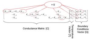
As described in [2], an energy balance can be applied to each node and equations that relate the node temperatures to their thermal resistances can be generated. The equations are written using values of conductances, K, which are the inverses of the thermal resistances, R (Ki-j = 1/Ri-j). The individual energy balance equations can be written into matrix form with the conductance matrix, [C], multiplied by the temperature vector, {T}, being equal to the boundary condition vector, {Q}, which represents the effects of dissipated power and reference temperature. Figure 2 shows this matrix equation.
The equation in Figure 2 is identical to equation (11) in Ref. [2] except that that it includes diagonal terms (K1-2, K2-2, etc.) as well as K1-4, q2 and q3. These terms were not shown in the Ref. [2] equation because they are all equal to zero for the problem being discussed. They are included in Figure 3 however to illustrate general characteristics by which the conductance matrix and boundary condition vector can be generated. These are summarized in Table 1.
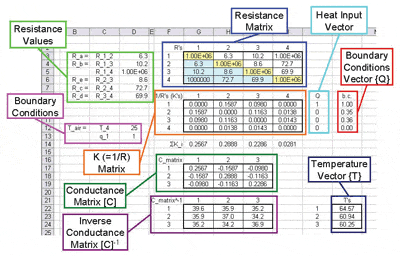
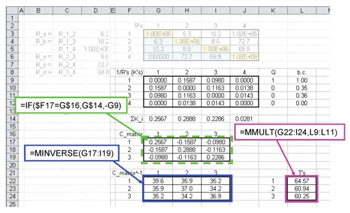
To solve for the nodal temperatures, the inverse of the conductance matrix is multiplied by the boundary condition vector, i.e., {T} = [C]-1 {Q}. A spreadsheet can not only solve this matrix equation, but can also be used to efficiently set up the matrices in a logical and understandable format. Figure 3 shows a portion of a spreadsheet that was set up to solve the thermal resistance network problem described in [2]. The figure is annotated to show what is accomplished in various regions in the spreadsheet1, starting on the left side where resistance values and boundary conditions are defined. These individual resistances are used to generate the resistance matrix to then define the K matrix. The rules in Table 1 are then used to generate the conductance matrix, [C] and the boundary condition vector, {Q}. Once [C] and {Q} have been calculated, the spreadsheet solves for nodal temperatures using matrix operations. The following paragraphs describe the specific Excel functions used to perform these steps.
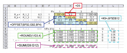
To generate the resistance matrix, one must first define an n x n array of cells, in which n is the total number of nodes. Node number labels next to the left edge and above the array are used to define the location of the resistances. In the resistance matrix shown in Figure 4, the upper-right hand cells are defined by referencing the corresponding cell in the list of resistances (for example R1-2 in the matrix points to cell D3 in the list of resistances). The diagonal terms in the resistance matrix (in yellow) are set to have essentially infinite thermal resistance of 1e6. Similarly, since Node 1 and Node 4 are not connected, the thermal resistance between them is also set to 1e6.
The resistance matrix is symmetric (the resistance between nodes 1 and 2, R1-2 is identical to the resistance between nodes 2 and 1, R2-1). The cells in bottom, left-hand portion of the matrix are generated using the =offset(reference cell, r, c) function, which returns the value of the cell that is r rows below and c columns to the right of the reference cell2. Through the appropriate use of absolute and relative references3, a single equation can be input and copied to fill the rest of the lower, left-hand portion of the resistance matrix.
Once the resistance matrix has been established, the values of K can be determined by finding the inverse of each R-term. The function =round(value, z), rounds the result to z decimal places. In this case, a somewhat arbitrary value of z=4 was assigned; this rounded the values of K to 4 decimal places and caused the approximately infinite thermal resistance values of 1e6 to become truly infinite, as their reciprocals were rounded to 0 using this function. Figure 4 also shows that the sums of the K-values for each node were calculated using the =sum() function to add up the four terms in each node’s column.
Finally, the boundary condition vector terms were calculated by adding the heat input value for each node (which were entered manually as the Heat Input Vector in Figure 3) to the reference temperature (T4) multiplied by the thermal conductance (K) between the node and the reference temperature. If multiple reference temperatures are defined in a system, such as a system that is cooled internally by air at a different temperature than the outside air temperature, the boundary condition vector would include the sum of each reference temperature multiplied by the corresponding K value.
| 1. | Diagonal terms (K1-1,K2-2, etc.) and resistances between nodes that are not connected are designated as having infinite thermal resistance and the conductance is zero. |
| 2. | All non-diagonal terms in the conductance matrix are equal to –Ki-j, i.e. -1/Ri-j. |
| 3. | On the diagonals, the terms in the conductance matrix are the summation of all Ki-j values for thermal resistances connected to that node. |
| 4. | The terms in the boundary conditions vector are defined as the heat dissipation at the corresponding node added to the reference temperature (or temperatures) multiplied by the conductance between that node and the reference temperature(s). |
Table 1. Rules to Generate Conductance Matrix and Boundary Condition Vector
The equations for calculating and utilizing the conductance matrix, [C], are shown in Figure 5. Since Node 4 is a defined boundary condition, it is not included in [C], the terms of which are determined using the =if(statement, true, false) function. Using the appropriate absolute/relative references4, the =if() function determines that a cell is along the diagonal if its row number equals its column number. If the cell in the conductance matrix is on the diagonal, its value is equal to the sum of conductance values for that node (ΣK_i). If a cell in the conductance matrix is not on the diagonal, its value is equal to –K for that cell. Again, this function is written in such a manner that it is entered once and then copied to fill the rest of the conductance matrix.
Once the conductance matrix has been defined, its inverse can be calculated using Excel matrix functions5. Matrix functions create arrays of cells, the size of which depend on the matrices that they are processing. To calculate the inverse of a matrix, select a separate set of cells that have the same number of rows and columns as the original matrix. Then type the function =minverse (reference_cells), in which reference cells is the entire range of the matrix to be inverted. At this point, do not simply ‘Enter’ the function but instead use ‘Ctrl-Shift-Enter’ to define it as a matrix function. This will generate the inverse conductance matrix in the cells that were initially selected. The node temperatures can then be calculated by multiplying the inverse conductance matrix with the boundary conditions vector using the =mmult(inverse conductance matrix, boundary conditions vector). This function, like =minverse(), is a matrix function so three cells (for the three nodes) must be highlighted and the equation must be entered using ‘Ctrl-Shift-Enter’.
In conclusion, while spreadsheets may not be the most efficient method for solving matrix equations, they can be an effective alternative to other methods that may not be as accessible to many engineers. Part 2 of this series will discuss application-specific issues for creating and adding thermal resistances as well as describe an actual industry analysis that used the thermal resistance network approach to assess an electronics system.
REFERENCES
Lasance, C., “Thermal Resistance: An Oxymoron?”, ElectronicsCooling, May 1997 (https://electronics-cooling.com/1997/05/thermal-resistance-an-oxymoron/).
Simons, R., “Using a Matrix Inverse Method to Solve a Thermal Resistance Network”, ElectronicsCooling, May 2009 (https://electronics-cooling.com/2009/05/using-a-matrix-inverse-method-to-solve-a-thermal-resistance-network/)
http://orion.math.iastate.edu/mathbus/sp/current/excel/tutorial2.xls
Ross Wilcoxon can be reached at rkwilcox@rockwellcollins.com.


