Calculation Corner: Measuring Heat Load to Water in a Rear Door Heat Exchanger Application

For almost 10 years now, the increasing heat loads in data centers have been recognized as a growing problem [1]. One of the approaches that has been effective in attacking this problem is the introduction of a water-cooled heat exchanger at the rear of a rack [2-5]. Using this approach, a part or nearly all the heat load absorbed by air passing over the heat dissipating electronics is transferred to water, which can carry the heat away much more efficiently than air. It also significantly reduces or eliminates the problem of hot air recirculation [6].

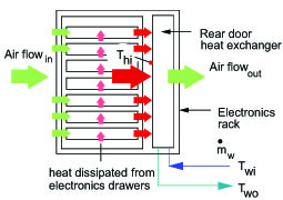
A simple schematic of a water-cooled heat exchanger mounted at the rear of an otherwise air-cooled rack is shown in Figure 1. Fans mounted in the electronics drawers pull air in from the front of the rack. As the air passes over the power dissipating components, heat is transferred to the air. However, before leaving the rack the air flows over a water-cooled, finned-tube heat exchanger mounted at the rear of the rack. Since the water entering the heat exchanger is at a lower temperature, T_wi , than the air, T_hi, entering the fin passages, heat is transferred from air to the water. Air leaving the rack will then be at a lower temperature than without the aid of the heat exchanger, thus reducing the heat load on the computer room air conditioning (CRAC) units. As one might expect, in such applications it is desirable to determine the amount of heat actually transferred to water. In principle, this may be done by measuring the water mass flow rate, _w, through the heat exchanger, and the temperatures of the water entering, T_wi, and leaving, T_wo, the heat exchanger. If the preceding quantities are known, the rate, q,  at which heat is transferred to water is given by

where c_p is the specific heat of water. The same equation would apply to a water-to-water heat exchanger as is used in some applications [5] to reject heat from system cooling water to customer side cooling water.

For purposes of illustration we will assume that the water flow rate through the heat exchanger is 75.7 liters/minute (i.e. 20 gpm) and the heat load to water is 20 kW. Using a specific heat of 4.179  kJ/kg-K for water  and equation [1], we can determine that the temperature rise in the water flowing through the cold side of  the heat exchanger would be 3.8^oC. So, if water on the cold side enters the heat exchanger at 25^oC, it will leave at 28.8^oC.  Now, let us change the situation and assume that we measure the water flow rate through the cold side of the heat exchanger to be 75.7 liters/minute and measure an inlet water temperature of 25^oC and exit water temperature of 28.8^oC. Based upon the preceding discussion, we know that if we use equation [1] we will find that the heat load transferred out of the heat exchanger is 20 kW. However, the real world is not quite that simple. In the real world there will be uncertainties in both our measurement of the water flow rate and the water temperatures in and out of the heat exchanger. So the question becomes, how can we bound or estimate the resulting uncertainty in our heat load measurement?

One way we could estimate extreme upper and lower bounds on the heat load measurement is to combine the upper and lower extremes of our measured values in equation [1]. However, to do this we must have some knowledge of the tolerances on our measured flow rate and temperatures. Again, for purposes of illustration, let us assume that the tolerance or uncertainty in the flow rate measurement is +/- 1.89 liters/minute (+/- 0.5 gpm) and the tolerance on the inlet and exit water temperature measurements is +/- 1^oC.

To obtain the upper limit on the measured heat load we can use the following equation

in which the constant a is equal to _wc_p/G and G is the water flow rate in liters per minute. For water, the constant a, will have a value of 69.35 W/liter/min/^oC.  The Δ quantities are the tolerance on measured flow rate and temperatures.

In a similar manner, the lower limit on the measured heat load is given by

Entering the assumed measured values of water flow rate (75.7 liters/minute), inlet and outlet temperatures (25^oC and 28.8^oC) and their respective tolerances, we calculate a maximum value of heat load of 31.2 kW and a minimum value of 9.2 kW compared to the nominal value from equation [1] of 20.0 kW. Clearly, these limits are extreme values and we would not expect the possible variations in our measurements to gang up on us in so malicious a manner. Nonetheless, we are left to wonder how we might obtain a more reasonable estimate on the likely bounds on our heat load measurement.

To do this, we must make a brief venture into the world of statistics. As we all know, just about anything we produce, or measurement we make, will exhibit some variation about a mean (or nominal) value. The distribution of these values about the mean quite often follows a normal distribution. A normal distribution is characterized by two parameters – its mean (µ) value and standard deviation (σ). The mean is simply the average value of the total population of values constituting the distribution. The standard deviation is a measure of how spread out or narrow the distribution of values in the population is. Mathematically, the standard deviation is the square root of the variance (σ²), which in turn is the average value of the squared differences from the mean.

In a normal distribution plus or minus one standard deviation about the mean encompasses 68.2% of the population, plus or minus two standard deviations encompasses 95.5 % of the population, and plus or minus three standard deviations encompasses 99.7% of the population. For most practical purposes three standard deviations may be considered to encompass 100% of the population. So, we may consider that the tolerance on our flow and temperature measurements is equivalent to three standard deviations.

Then

For the example we have been considering, the nominal measured values of flow rate, inlet water temperature and outlet water temperatures are respectively 75.7 liters/minute, 25^oC and 28.8^oC. Based upon the measurement tolerances of  +/- 1.89 liters/minute on flow rate and +/- 1^oC on temperature, using equation [4] the standard deviations on these measurements are 0.63 liters/minute and 0.333^oC/W respectively.

However, what we need to find is the standard deviation, σq on the heat load, σ_q , as calculated using equation [1] and the nominal measured values of flow rate, G , and temperature, T_wi and T_wo.  To do this we will use a modified form of equation [1] to calculate the mean or nominal heat load

where a is the same as used in equations [2] and [3].

Then after applying the mathematical rules for combining products and difference of random variables and some algebraic manipulation, it can be shown that the variance and standard deviation of the measured value of heat load is

and

where ΔT is the difference between the measured water temperatures T_wo and T_wi. Entering the various values under discussion in equation [7], the calculated standard deviation of the heat load measurement is 2480 W. Since two standard deviations would capture 95 % of the population, it would be reasonable to conclude that the true value of heat load is most likely within the range of 15 to 25 kW, compared to a range of 9.2 to 31.2 kW calculated using the min and max equations [2] and [3].

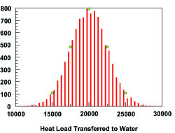
In order to check the validity of equation [7], a Monte Carlo simulation was set up to model equation [1] statistically. To do this, a nominal set of values is selected to simulate measured flow rate, inlet water temperature and exit water temperature that would give a particular value of heat load (in this case 20 kW). Then the standard deviation of each of the assumed measured values is used in concert with a random number generator and the assumed probability distribution (in this case a normal distribution) to generate random measurement values to enter in equation [1] to create a randomly generated value of heat load. This is done many times (in this case 10,000 times) to create the distribution of measured heat load values. The distribution obtained for the example under consideration is shown in histogram form in Figure 2. The vertical axis displays the number of occurrences of the heat load values displayed on the horizontal axis. The standard deviation, s_q, on heat load can be calculated from the total population or set of calculated heat load values using

where q_i are all the calculated values of q, is the average of all these values and n is the population size which is the number of Monte Carlo runs.

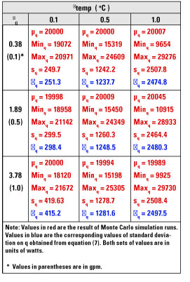
To demonstrate the validity of equation [7] numerically, Monte Carlo simulation runs were made over a range of standard deviations in temperature measurement (0.1, 0.5 and 1^oC) and in flow measurement (0.38, 1.89 and 3.78 liters/minute) and the corresponding standard deviations in the simulated measured heat load was calculated. The simulation was based upon a heat load of 20 kW and a water flow rate of 75.7 liters/minute as discussed earlier in this article. A similar set of calculations was made using equation [7]. A comparison of the standard deviation values obtained by each method is shown in Table 1. From Table 1 it can be seen that the standard deviation calculated from the Monte Carlo simulation results and equation (7) are very nearly the same, differing at most by less than 1.5%.

Thus equation (7) can be very helpful in evaluating the effect of flow and temperature measurement uncertainties on the uncertainty in measurement of heat load on a heat exchanger, as well as to provide upper and lower bounds on the probable value of the heat load measurement.

References

[1]      Schmidt, R.R. “Hot Spots in Data Centers.” ElectronicsCooling, August 2003.

[2]      Whitenack, K. “Liquid Cooling for Datacom Equipment Centers.” ElectronicsCooling August 2008.

[3]      Schmidt, R.R. “Liquid Cooling is Back.” ElectronicsCooling, August 2005.

[4]      LaPlante, S.R., Aubry, N., Rosa, L., Levesque, P., Porter, D., Cavanaugh, C., and Johnston, J. “Liquid Cooling of a High-Density Computer Cluster.” ElectronicsCooling, November 2006.

[5]      Campbell, L., and Ellsworth, M.J. “Back to the Future With a Liquid Cooled Supercomputer.” ElectronicsCooling, August 2009.

[6]      Simons, R.E. “Using a Simple Air Recirculation Model to Explore Computer Rack Cooling.” ElectronicsCooling, February 2007.