The first article in this series on spreadsheet based thermal resistance network analysis [1] described a procedure for using Microsoft Excel to solve a thermal resistance network by applying matrix analysis. That article assumed that the values of the thermal resistances between nodes were both known and fixed. This article presents methods for simplifying the process of incorporating values into the thermal resistance matrix and compares the results of a thermal resistance analysis and actual test data on a military electronics pod.
A thermal resistance network analysis is based on the idea that a system can be divided into a number of discrete nodes that are interconnected through thermal resistances. If the thermal path between two nodes is primarily one-dimensional conduction or convection, the thermal resistance can be calculated as Rcond = L/kAcross or Rconv = 1/hAsurface, respectively [2], where = L is the distance between nodes, k is the thermal conductivity of material between the nodes, Across is the cross sectional area of material between nodes, h is the convection coefficient of the solid node (the other node being a fluid) and Asurface is the surface area from which heat is convected. The convection thermal resistance can also be applied to systems with contact between two surfaces by replacing the convection coefficient with a contact resistance [3]. Many papers, such as [4-8] have described methods to calculate specific thermal resistances for electronics packages, heat sinks, spreading, packages on circuit boards, etc.
Once the nodes of a system have been defined, the resistances between them can generally be estimated using these various equations and entered into a resistance matrix such as that described in [1]. One approach for inputting these values into the matrix would be to separately calculate their values using design parameters and directly type them into the correct cell in the spreadsheet. This approach however, negates one of the primary advantages of using spreadsheets in solving a resistance network – namely the ability to easily change design parameters, such as dimensions and material properties, to assess their impact on overall thermal characteristics.
A somewhat better approach is to enter equations, which refer to cells in the spreadsheet for design parameters in the appropriate cells in the thermal resistance matrix. This may be a reasonable approach if the thermal resistance circuit only includes a few nodes and there are relatively few terms in the resistance matrix. However, if the model includes a large number of nodes, the analyst will soon find that a significant amount of time is required to type in equations (and correspondingly, the likelihood of incorrectly entering an equation will grow). As shown in [1], the resistance matrix will have N x N cells, where N is the number of nodes. The diagonal terms of this matrix are ignored (nodes do not conduct heat to themselves) and since the matrix is symmetric only half the remaining resistance terms must be entered. If 10 nodes are included in a model, there are therefore [10*(10-1)/2 = 45] total thermal resistances in the model. As the size of the resistance model grows, the number of thermal resistances in the model increases; for example, a circuit with 20 nodes could have up to 190 thermal resistance terms. Accurately entering this many values or equations into a spreadsheet would likely require effort significant enough to overwhelm the benefits of using spreadsheet analysis in the first place. However, standard spreadsheet functions can be incorporated to greatly reduce the effort required to complete the resistance matrix. Two approaches for simplifying the entry of resistance values are described: a lookup table and direct calculation.
Lookup Table
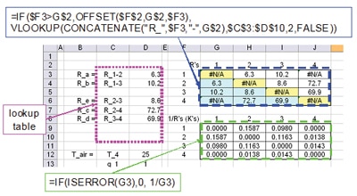
One approach that can simplify entering resistance values is to create a list of the resistances in a lookup table. The table utilizes a naming convention based on unique node names or numbers (such as R_1-2 corresponding to the thermal resistance between nodes 1 and 2). The node names or numbers can then be incorporated into a header row and column of the resistance matrix and used to generate a name using the @concatenate() function, which creates a text string by combining individual text strings. For example, a text string of R_1-2 can be generated with the function @concatenate(“R_”,$B5, “_”,D$3) if cell B3 has a value of 1 and cell D3 has a value of 2. This text string can be generated in the resistance matrix and used with the @vlookup() function to identify the correct resistance value in a lookup table. The @vlookup(value, array, column #, range lookup) function looks for a ‘value’ in the first column of an ‘array’ and returns the value in the ‘column #’ of the same row of the array. If the data in the first column of the array are not necessarily sorted in order, the ‘range lookup’ should be set to “false”. For example, Figure 1 shows a modified version of the spreadsheet presented in [1] in which the cells in the resistance matrix all include the same equation that has been copied to fill the array. As in [1], an @if() function is used to determine if a cell is below the diagonal of the matrix and if it is, the value in that cell is set to be the value of its symmetric cell (i.e., R_2-1 = R_1-2) using the @offset() function. For the cells that are on or above the diagonal of the matrix, the @vlookup() function is used to determine resistance values for a combination of node numbers by searching the lookup table. The resistance name used in the @vlookup() search, such as R_1-2, is generated with the @concatenate() function that uses the node numbers designated in Column F and Row 2. Note that the ‘range lookup’ is set to FALSE and the size of the lookup table used by @vlookup() includes blank cells so that additional resistances could be added to the table if needed. Also note that the absolute and relative reference defined by including the “$” symbol in the appropriate column and/or row reference in the cell reference is critical to generating an equation that can be entered once and copied throughout the resistance matrix.

The equation used to determine the individual conductance values (K = 1/R) was modified relative to what was presented in [1] to account for the impact of using the @vlookup() function. When the @vlookup() function does not identify a corresponding cell, such as those on the matrix diagonal: R_1-1, R_2-2, etc., a value of #N/A is returned. If the lookup table accounts for all nodes that are thermally connected, then any nodal resistance not included on it would correspond to nodes that aren’t connected, i.e. infinite R and K = 0. The equation in the K matrix uses the @iserror() function to identify those cells in the resistance matrix that have R = #N/A and sets the value of K to be 0. Cells that have a finite resistance are used to calculate the conductance values using the inverse of the corresponding cell resistances.
Direct Calculation
As mentioned previously, a number of the thermal resistances between nodes can be expressed in terms of one dimensional conduction (R = L/kA) or convection (R = 1/hA). In many cases, some of these parameters (such as k, h or A) can be defined directly for a given node or a combination of node properties (for example in conduction, L could be the physical distance between two nodes). If a thermal resistance can be directly calculated from nodal properties, these properties can be written into header columns and rows corresponding to the resistance matrix. Equations in the cells that make up the thermal resistance matrix can then calculate the thermal resistance for a given node combination by directly referencing the properties written to these header rows and columns.
The application of this approach to a system with a relatively large number of nodes is illustrated in the analysis on an electronics missile pod (see Figure 2). In this system, some of the existing electronics modules were being replaced with devices with higher power dissipation. In the early module design and system integration definition, a number of design parameters were not finalized, making the generation of a solid model for thermal analysis quite challenging. However, an understanding of the pod thermal capabilities was needed to adequately assess the design risk, so a nodal analysis of the pod was conducted to identify the thermal performance of the pod and quantify the impact of various design uncertainties.

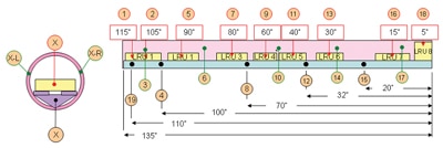
The electronics missile pod included a mounting rail to which the line replaceable units (LRUs) are attached. This rail slides out of the round tube for maintaining the LRUs and is attached to the tube at a number of discrete locations. A total of eight power dissipating LRUs were attached to the rail. A conceptual sketch of the electronics pod, with side and cross section views that indicate the locations of numbered nodes (in inches), is shown in Figure 2. Three types of nodes were included in the thermal model: red nodes indicate the locations of the LRUs, black nodes indicate the locations at which the mounting rail was attached to the outer tube and green nodes indicate regions on the tube midway between the rail mounting locations. The model was set up with nodes on each side of the tube to allow solar loading to be applied to only one side of the tube.
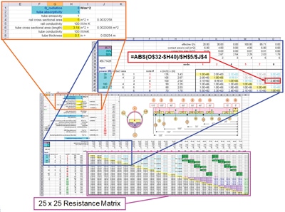
In all, a total of 25 nodes were defined in the thermal analysis of this system. As discussed previously, this large of a system would normally not be suitable for a nodal analysis due to the large number of thermal resistances that had to be defined (25*(25 1)/2 = 300). However, in this case the distances between nodes and the convection areas from the external surfaces could be defined as functions of the node location. Therefore, cells in the columns next to the resistance matrix were populated with data that specifies node location and heat transfer contact areas. The @offset() function was used to transpose this data to rows above the resistance matrix and equations that referenced these terms were used to calculate thermal resistances in individual cells in the resistance matrix. In all, seven different types of thermal resistances were included in the model: combined contact resistance between the modules and rail and conduction along the pod rail, conduction along the pod rail, convection from modules to inside of tube, contact between rail & tube with conduction along tube, conduction between halves of tube, convection and radiation from the tube to the surroundings, and conduction along the tube.

Once one of these resistances had been typed into an appropriate cell in the matrix, it could be copied into the other cells corresponding to combinations of nodes that were thermally connected with the same type of resistance. Each type of resistance was assigned a specific formatting (font color and cell background) to simplify visual inspection of the matrix so that the appropriate resistances could be assigned to a given cell. Figure 3 shows a screenshot of part of the spreadsheet that illustrates the rows and columns used to calculate individual resistances and the use of cell formatting to differentiate the different types of resistances used in the matrix. For example, Figure 3 highlights the cell for the resistance between nodes 4 and 8, which accounts for conduction between two nodes on the rail. This was calculated using L/kA where L was the distance between the locations of the nodes, k was the thermal conductivity of the rail (defined in cell $H$5) and A was the cross sectional area (defined in cell $J$4). The locations of the nodes were referenced from data in row 32 and column H, which were fixed by the $ symbol, and the absolute value function, =abs(), ensured that the resistance would be positive regardless of which location had a larger magnitude. After this equation was input once, its formatting was set to black font/gray background and it was copied to all cells in the matrix that corresponded to resistances that represented conduction paths between rail nodes. Note that all node locations, contact areas, material properties, LRU powers, etc. shown in Figures 2 and 3 have been changed for this article to protect any sensitive information.
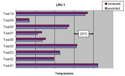
The details of the thermal analysis of the missile pod are beyond the scope of this article. The main goal of discussing this analysis was to illustrate how resistances can effectively be calculated in the thermal resistance matrix and that the resistance network can be quite accurate. Figure 4 shows a comparison between temperatures predicted with the matrix analysis and the results of lab testing performed with the pod operating under a range of power dissipation conditions in some of the LRUs.

Final comments
As noted by Henry Petroski, “To Engineer is Human” [8]; therefore it is not unusual that the analyst may recognize that additional nodes or resistances may be needed after the thermal resistance matrix has been initially created. Adding or removing a thermal resistance to or from an existing model is trivial; it simply requires that the appropriate cell in the resistance matrix be updated. However, adding an additional node requires significant alterations to the entire spreadsheet and recreating the matrix equations. This can be avoided if the original matrix includes ‘dummy’ nodes that are initially only thermally connected to one other node (such as the ambient). If the analyst later recognizes that additional nodes should be included in the analysis, the dummy nodes can be used and the resistance matrix can be modified accordingly.
As a final comment, the matrix solution is certainly not the only approach that can be taken to solve for nodal temperatures. MS Excel has a number of tools, such as Solver, that can be used in place of the method outlined in [1]. Different approaches each have their own advantages and disadvantages. In many cases, the most important factor is simply the approach with which the analyst is most comfortable. Regardless of whether matrices, ‘Solver’, or some other method is used for solving the resistance network, minimizing the data entry for generating such a matrix can greatly simplify the analysis and reduce errors.
The next article planned for this series will discuss methods for including non-linear effects, such as radiation and temperature dependent material properties or convection coefficients, in the matrix analysis. It will also describe methods for extending the basic steady-state, fixed resistance analysis to address issues such as uncertainty (using a Monte Carlo analysis) and to perform a transient thermal analysis using a simple numerical integration approach.
References
1. Wilcoxon, Ross “A Spreadsheet Based Matrix Solution for a Thermal Resistance Network: Part 1”, ElectronicsCooling, September 2010
2. Vincent Manno, “Integrated Thermal Network Models are Still Useful, ElectronicsCooling, September 1997
3. P. Teertstra, M. M. Yovanovich and J. R. Culham, “Calculating Interface Resistance”, ElectronicsCooling, May 1997
4. B.M Guenin, R.C. Marrs, and R.J. Molnar; “Analysis of a thermally enhanced ball grid array package”, Components, Packaging, and Manufacturing Technology, Part A, IEEE Transactions on, Vol.18, No.4, pp 749-757, 1995
5. Robert Simon, “Estimating Parallel Plate-Fin Heat Sink Thermal Resistance”, ElectronicsCooling, February 2003
6. Robert Simon, “Simple Formulas for Estimating Thermal Spreading Resistance”, ElectronicsCooling, May 2004
7. Bruce Guenin, “Heat Spreading Calculations Using Thermal Circuit Elements”, ElectronicsCooling, August 2008
8. ElectronicsCooling Editors, “Convection and radiation heat loss from a printed circuit board”, ElectronicsCooling, September 1998
9. Henry Petroski, “To Engineer is Human”, St. Martin’s Press, New York, 1985


