Calculation Corner: Spreadsheet-based Matrix Analysis – Extension to Transient Analysis

by Ross Wilcoxon, Ph.D., Associate Technical Editor

Over the years, a number of articles [1-3] published in ElectronicsCooling have described the use of thermal resistance networks to analyze electronic systems.  The analysis of a thermal resistance network begins by defining discrete nodes that are connected with resistors, with the magnitude of a flow between nodes defined by the configuration and the values of the individual resistors.  In a thermal analysis, the nodes represent individual regions of the system that are each assumed to have a uniform, or representative average, temperature within the region, while the resistances are the thermal resistances between the nodes.  This article describes how a thermal resistance network analysis for determining steady state temperatures can also be used to predict transient temperatures.

As described in [1], an inverse matrix analysis is a method that can be used to solve for the heat flows and nodal temperatures in a thermal resistance network with known boundary conditions.  Reference [2] describes a method for solving a given thermal resistance matrix using a spreadsheet, and automated methods for generating a resistance network in spreadsheets are outlined in [3].

To briefly review how a thermal resistance network is generated and analyzed, let us consider four nodes that are connected to each other with thermal resistances, with two of the nodes connected to the ambient air temperature (T4), as illustrated in Figure 1.  This network represents heat transfer in a single board-mounted electronic component described in [1,2], with the heat dissipating die designated as node T1.

 

 

 

 

 

 

 

 

 

 

 

 

 

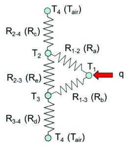
Under steady-state conditions, the energy that enters each node is equal to the energy that leaves it.  The energy balance on node 1 can be written as:

 (1)

 

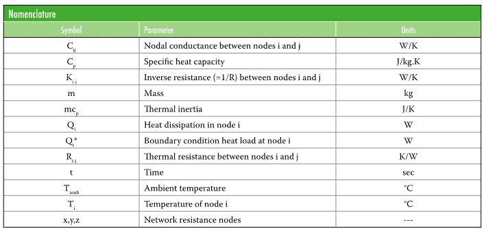
where Q is the external heat input to node 1 (i.e. power dissipation), T_x is the temperature of node x, and K_x-y is the thermal conductance between nodes x and y, i.e. the inverse of the thermal resistance.

For steady state conditions, the temperature does not change over time () and an energy balance can be applied to each body (i.e. node) with the three resulting equations written in matrix form:

 

(2)

 

 

where Q_i* = Q_i + T_amb/R_i-amb, T_amb is the ambient temperature, and R is the thermal resistance between the node and the ambient temperature.

Using the inverse matrix approach, the temperatures can be determined for a given set of specified boundary conditions (i.e. heat dissipation (Q) values and one of the nodal temperatures).  Equation (2) can be re-written as:

 

 

(2a)

 

where , and i and j are nodes in the resistance network.

 

TRANSIENT SOLUTION

The thermal resistance matrix solution can be extended to more complex systems with a larger number of nodes, and can be used to determine the steady state temperatures of a nodal system – assuming that the resistances between the nodes can be determined with sufficient accuracy.  However, as presented in [1-3], it does not provide a method for assessing the transient behavior of a system.  The transient response of a node can again be determined by applying an energy balance to it, but in this case it is recognized that its temperature changes with time, as shown in Equation (1).

This same energy balance can be applied to each node in the thermal resistance network that includes thermal resistances between nodes and values of thermal inertia (mc_p) for each node.  A number of approaches can be used to solve the set of equations generated when Equation (3) is applied to each node in the network.  For example, Guenin [4,5] compares the predictions of finite element modeling (FEM) to those of an analytical multi-stage resistor/capacitor network.

This article describes an alternative approach, using a simple numerical integration, for determining the transient behavior of a thermal resistance network solved using a spreadsheet analysis.  The primary advantages to this approach are that it can be added to a steady state analysis by using the same conductance matrix, and that it is relatively straightforward to account for power dissipation values that change with time and/or temperature.

As shown in Equation (3a), Equation (1) can be rewritten with finite changes in temperature and time, and is sufficiently accurate as long as the difference in time (∆t) is small^[1].  Equation (3a) can be rearranged into Equation (3b), in which T_{i, old} is the temperature of a node at a given time, and T_i,new is the temperature one time step, ∆t, later:

 

(3a)

 

 

 (3b)

 

 

It is apparent from comparing Equations (3b) and (2) that the conductance terms needed to solve for a temperature change are present in the conductance matrix used for the steady state analysis.  If a spreadsheet has already been created to solve the steady state temperatures using an inverse matrix approach, the conductance matrix can also be used for transient analysis.  This is relatively straight forward, particularly if one uses a somewhat convoluted function to simplify the conductance matrix.

To illustrate how to add a transient solution to an existing inverse-matrix resistance network solver, we will consider the four node model shown in Figure 1.

¹How “small” ∆T needs to be make the analysis “reasonably accurate” depends on the particular system being analyzed. The mass and specific heats of nodes and the rate at which power dissipations change over time can all influence how small of a time step is needed.  If predicted results do not change significantly when the time step is reduced, the time step is probably sufficiently fine.

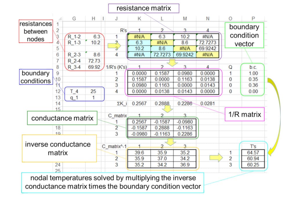
Figure 2 shows a matrix solution formulated in a spreadsheet for determining the steady state temperatures of the network shown in Figure 1.

 

This analysis can be extended to find a transient solution as shown in Figure 3.  This analysis begins by defining a time step value (shown in cell Q4) and defining columns for the power dissipation in each node (columns S, T and U).  The transient time (column W) starts at 0, at which the nodes are all assumed to be at ambient temperature, T4.  For this analysis, values of thermal inertia (mc_p) of 0.5, 0.3, and 1.1 J/K were applied to nodes 1, 2, and 3, respectively (shown in cells X2 through Z2).  These particular thermal inertia values were arbitrarily selected to allow the process to be demonstrated.  The effects of ambient temperature were calculated in cells X1 through Z1 by multiplying the value of 1/R between each node and ambient times the ambient temperature.

 

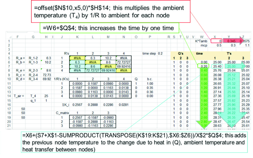
The somewhat convoluted function previously alluded to, was entered into cell X7 to calculate the temperature of node 1 after the passage of one time step.  This involved applying equation (3b) by adding the previous temperature in that node to the sum of: the heat dissipated in the node (in Cell S7), plus the value of K_1-ambient * T_ambient (Cell X$1), plus each nodal temperature (at the previous time step multiplied by its corresponding value in the C matrix (i.e. conductance matrix); this sum was divided by the value of mc_p (X$2) and multiplied by the time step ($Q$4).  The ‘TRANSPOSE()’ function converts the column of values in the C matrix into a row that can be multiplied by the row of previous temperatures using the ‘SUMPRODUCT()’ function [6], which multiplies corresponding components in the given arrays, and returns the sum of those products.

Through careful use of absolute and relative referencing (defined by whether a “$” sign is placed before a column and/or row reference), only three equations were typed into this portion of the spreadsheet and then copied to the rest of the columns or rows, as indicated in the block arrows.  Note that since the TRANSPOSE() function is an array function, the equation must be entered with a Ctrl-Shift-Enter rather than simply the Enter key.  Also, if changes are made to a cell with an array function, it may be necessary to firstly clear previous matrix equations from those cells before copying updated equations into them.

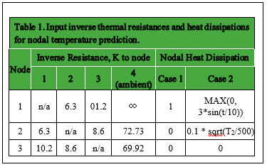
The resulting transient solution shows the temperature asymptote to the steady state temperatures of 64.6 °C, 60.9 °C and 60.3 °C for nodes 1, 2 and 3, respectively, that were predicted using the inverse matrix analysis, as shown in Figure 4.  The specific values for thermal resistances and heat loads used in this analysis, Case 1, and an additional analysis, are summarized in Table 1.

 

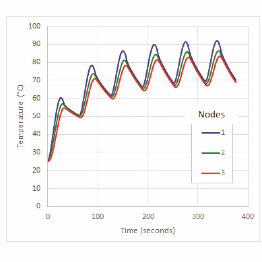
The spreadsheet could have been slightly simplified by using fixed values for the power dissipation for each node, rather than using constant values assigned to the three columns (S,T and U).  However, using the values in the individual columns does allow for the analysis to include temperature and/or time-dependent power dissipation.  For example, Figure 5 shows the transient temperatures for the same system when the power dissipation in node 1 was determined with the equation =MAX(0, 3*sin(t/10)), to simulate a pulsed power dissipation, and the power dissipation of node 2, which was 0 in the previous analysis, was defined as  0.1 * sqrt(T₂/500), to simulate a temperature dependent power dissipation.  These equations were easily implemented into the existing columns for power dissipation.

 

 

FINAL COMMENTS ON SPREADSHEET-BASED ANALYSIS

Spreadsheets are wonderful tools that can be used to analyze a wide variety of scientific problems.  Even their most ardent supporters, however, will grudgingly admit that at some point there are better tools for analyzing complex systems.  If a thermal analysis requires more than a dozen nodes to sufficiently describe a resistance network, it may be time (or past time) to consider using a dedicated analysis tool such as FEA software.  As the number of cells in a spreadsheet grows, the chances for mistakes in typing, etc., grow and the savings accomplished with a “quick and dirty” analysis can ultimately be quite expensive.  Using “cookbook” approaches, such as what has been described in this article, can reduce the risk of user errors by limiting the number of different equations that need to be typed into the spreadsheet.  However even with these approaches, the spreadsheet analyst needs to be willing to admit when the complexity of a particular analysis has moved to the point at which other tools are more appropriate.

With that said, spreadsheet-based analysis can be extremely useful and can often accelerate the understanding of a situation.  An additional advantage of spreadsheets is their transportability.  In this author’s experience, there have been a number of cases in which customers (both internal and external) requested a tool to help them understand the impact of different decisions, rather than a static analysis of a given set of design decisions.  Many of those customers did not have access to the necessary FEA tools or the knowledge to use them; however they all knew how to use a spreadsheet.

 

References

[1] Simons, R., “Using a Matrix Inverse Method to Solve a Thermal Resistance Network,” ElectronicsCooling, June 2009, https://electronics-cooling.com/2009/05/using-a-matrix-inverse-method-to-solve-a-thermal-resistance-network/, accessed August 11, 2016.

[2] Wilcoxon, R., “Calculation Corner: A Spreadsheet based Matrix Solution for a Thermal Resistance Network: Part 1,” ElectronicsCooling, September 2010, https://electronics-cooling.com/2010/09/calculation-corner-a-spreadsheet-based-matrix-solution-for-a-thermal-resistance-network-part-1/, accessed August 11, 2016.

[3] Wilcoxon, R., “Spreadsheet Based Thermal Resistance Analysis Part 2: Generating the Thermal Resistance Matrix,” ElectronicsCooling, June 2011, https://electronics-cooling.com/2011/06/spreadsheet-based-thermal-resistance-analysis-part-2-generating-the-thermal-resistance-matrix/, accessed August 11, 2016.

[4] Guenin, B., “Calculation Corner: Transient Thermal Modeling of a High-Power IC Package, Part 1,” ElectronicsCooling, December 2011, https://electronics-cooling.com/2011/12/transient-modelling-of-a-high-power-ic-package-part-1/, accessed August 11, 2016.

[5] Guenin, B., “Calculation Corner: Transient Thermal Modeling of a High-Power IC Package, Part 2,” ElectronicsCooling, March 2012, https://electronics-cooling.com/2012/03/calculation-corner-transient-modeling-of-a-high-power-ic-package-part-2/, accessed August 11, 2016.

[6] Microsoft Excel, “SUMPRODUCT function,” https://support.office.com/en-us/article/SUMPRODUCT-function-16753e75-9f68-4874-94ac-4d2145a2fd2e, accessed August 11, 2016.

 

Contact Information

Ross Wilcoxon, Ph.D.,  |  Principal Mechanical Engineer
Advanced Technology Center  |  Rockwell Collins
400 Collins Rd NE, MS 108-101, Cedar Rapids, IA 52498, USA
Email: ross.wilcoxon@rockwellcollins.com