INTRODUCTION
The state of the art in performing thermal calculations in our industry is very advanced. However, how applicable the results of a calculation are to the real-world performance of a packaging or an active cooling component depends on the quality of the data characterizing these various components. In the real world of manufacturing, such characterization parameters can never be a single value, but are always rep-resented by a statistical distribution.
Thermal calculations performed by engineers in our industry most often deal with nominal values of performance parameters that represent the design objective for a particular component rather than the result of a rigorous statistical analysis of detailed test results of its actual thermal performance. This sort of model is referred to here as a “deterministic model” [1].
This practice does not adequately address the risk that a component or system will not meet its thermal performance objectives. This article discusses the use of the Monte Carlo Method in that regard. It provides a surprisingly efficient process for adapting a deterministic model to account for the statistical variability of manufacturing and operational parameters that have a significant effect on the operating temperature of critical electronic devices.
THERMAL MODEL
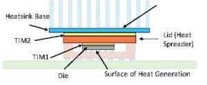
The system to be analyzed here and the thermal model characterizing it have been discussed in previous installments of this column [2, 3, 4]. It is depicted in Figure 1. It consists of a flip-chip package with a copper lid to which a heat sink is attached. The package design is representative of those used for high pin count, high power ICs, with dissipated power levels in excess of 50W. The dominant heat flow path is from the active surface of the die (facing the substrate), up through the silicon, through the TIM1 layer (TIM = thermal interface material), the copper lid, the TIM2 layer, and into the heat sink whence it transferred into a flow-ing air stream. The heat flow path through the substrate and into the PCB (printed circuit board) represents only a small fraction of the total dissipated heat and is neglected here.
The TIM1 and TIM2 layers account for most of the variability in the thermal resistance path between the chip and the air. This is due to their much lower thermal conductivity then the other components and the variability in their thickness.
Reference 2 presents the design assumptions and calculated thermal results for 36 different configurations, representing different heat sink width, base thickness, thermal conductivity, and effective heat transfer coefficient (representing the cooling effect of the heat sink fins at different assumed values of air velocity). Configuration #31 is assumed here. [Reference 4 deals only with Configuration #31. It provides the details of this configuration in a more readable form than Reference 2].
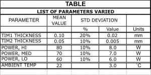
Table 1
FIGURE 1. Diagram of high-power package attached to a heatsink. Components in bold color are explicitly represented in the model. Those in a faint color are part of the physical assembly, but are not represented in the model.
For configuration #31, the calculated value of ΘJA = 0.87 ˚C/W. The assumed thickness and calculated thermal resistance for the two TIMs are as follows: TIM1: 0.1 mm, 0.296 ˚C/W; TIM2: 0.05 mm, 0.163 ˚C/W. Their combined thermal resistance is 0.46 ˚C/W and represents roughly 50% of the total thermal resistance. Variations in their thickness will have a significant effect on the ultimate value of ΘJA. The relationships between the thermal resistance of the TIM1 and TIM2 layers and their thickness are provided by the following two equations:
(1)
(2)
where the TIM thickness values, tTIM1 and tTIM2, are in mm units. HTA is defined as the Heat Transfer Area through TIM2 = 17.5 mm *17.5 mm = 306 mm2 [3,4]. The die area = 13 mm * 13 mm = 269 mm2. The TIM1 and TIM2 materials are silver-filled epoxy and a metal-filled grease, respectively. The thermal conductivity values, kTIM1 and kTIM2 are equal to 2 W/mK and 1 W/mK, respectively. The following expression provides the calculated value of ΘJA as a function of the newly calculated values of ΘTIM1 and ΘTIM2:
(3)
Note that when ΘTIM1, NEW and ΘTIM2, NEW are equal to their original values, ΘJA, NEW is equal to its original value also, as would be expected. The final junction temperature of the die is calculated using ΘJA, NEW, the dissipated power, and the ambient air temperature using:
(4)
STATISTICAL ANALYSIS OF VARIATIONS IN A SINGLE PA-RAMETER
The next step in this process is to quantify the variability in the thickness of the TIM1 and TIM2 layers. This would normally begin with the measurement of these parameters on a population of randomly selected parts from the manufacturing line.
The results would be plotted in the form of a histogram and an appropriate function fitted to the data. In most cases, a normal (or Bell Curve) distribution is found to be effective in representing the variations of data of this sort [5].
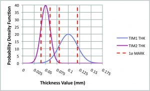
Figure 2a displays a graph containing two normal distributions, each representing the statistical variation of the thickness of one the two TIMs. The mean values and standard deviations of these curves are provided in the Table. The curves are produced in a spreadsheet using the function:
NORMDIST (Thickness, Mean Value, Std. Deviation, FALSE) (5)
In order to embed this function in a spreadsheet to generate the curves, a column of ascending thickness values needs be created. A second column is populated with the NORMDIST function, with the Thickness argument in each occurrence of the function linked to the appropriate thickness value in the neighboring column.
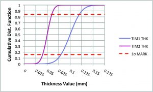
These curves are referred to as Probability Density Functions. Note that the distribution of the TIM2 thickness data is more peaked than for TIM1 due to having a smaller standard deviation (0.005 mm vs 0.02 mm). The dashed red lines mark the width of a single standard deviation on each graph. The graph in Figure 2b is displays the Cumulative Distribution Functions, based on the Probability Density Functions in 2a. Generally, a Cumulative Distribution Function is produced by a numerical integration of its respective Probability Density Function from minus infinity to plus infinity.
It provides a convenient means for determining the percentage of the total sample population having thick-ness values in an arbitrary range. The dashed red lines in the figure bracket a fraction of the total sample population equal to a single standard deviation or 68.3% of the total. These Cumulative Distribution Functions were generated in a spreadsheet using the function:
NORMDIST (Thickness, Mean Value, Std. Deviation, TRUE) (6)
FIGURE 2a and 2b. Statistical distributions of thickness values for TIM1 and TIM2 per the values of mean value and standard deviation listed in the Table. Dotted lines bracket a single standard deviation in the graphs.
APPLICATION OF MONTE CARLO METHOD
“Monte Carlo simulation is a type of simulation that relies on repeated random sampling and statistical analysis to compute the results. This method of simulation is very closely related to random experiments, experiments for which the specific result is not known in advance” [1].
The method requires the Inverse Cumulative Distribution Function to generate a randomly sampled population of thickness values consistent with the statistics in the original Probability Density Function. This inverse function has the following form in the spreadsheet:
NORMINV (Thickness, Mean Value, Std. Deviation) (7)
In a spreadsheet, this is accomplished by linking the Thickness argument in the spreadsheet NORMINV function to a cell containing the random number function divided by an appropriate constant; such as:
RANDBETWEEN (1,9999)/10000 (8)
Note that this function randomly generates numbers between and including the limits: 1 and 9999. After the division by 10,000, these limits become: 0.0001 and 0.9999.
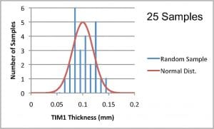
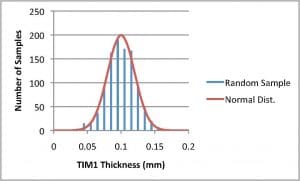
Figures 3a and 3b are the output of such a process. In 3a, only 25 random samples were generated. The resultant histogram deviates significantly from the Probability Density Function representing the original data. However, Figure 3b, the histogram generated using 1000 random samples tracks the original distribution well.
FIGURE 3a and 3b. Histograms generated using random sampled outputs from the Inverse Cumulative Distribution Function for TIM1: a) 25 samples; b) 1000 samples.
LINKING OF RANDOM SAMPLING OF TIM1 AND TIM2 THICK-NESS TO THERMAL MODEL
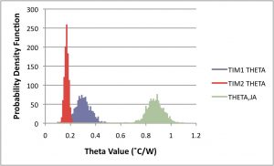
The histogram in Figure 3b can be used to generate an equivalent distribution of ΘTIM1 values by inputting each randomly sampled value of TIM1 thickness into Eqn. 1, and similarly for ΘTIM2. The resultant thermal resistance distributions are plotted in the graph in Figure 4.
Randomly selected pairs of sampled values of ΘTIM1 and ΘTIM2. from these distributions are input into Eqn. 3 to generate the associated distribution of ΘJA values, which is plotted on the right side of Figure 4.
FIGURE 4. Probability Density Function for calculations of: 1) ΘTIM1 and ΘTIM2, based on TIM1 and TIM2 thickness distributions and Eqns. 1 and 2. 2) ΘJA, based on ΘTIM1 and ΘTIM2 distributions and Eqn. 3.
CALCULATION OF JUNCTION TEMPERATURE DISTRIBUTION UNDER VARIOUS POWER ASSUMPTIONS
This final stage of the calculation is intended to predict the highest allowed power consistent with having a high probability that TJ will not exceed a specified value, which is normally chosen for reliability reasons. In this case, the TJ limit is set at a typical value of 90C. The Table displays the mean values and standard deviations for three different power distributions and also for ambient temperature. In order to implement the generation of different junction temperature distributions based on these different inputs the same procedure as before is implemented:
- Create the Probability Density Function using the appropriate spreadsheet function.
- Use the random number function as an input to the Inverse Cumulative Distribution Function, using the same mean value and standard deviation, to generate a random sampling of power levels and ambient temperatures.
- Input these values of power levels and ambient temperatures along with the previously generated distribution of ΘJA values into Eqn. 4.
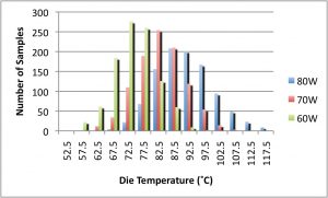
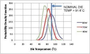
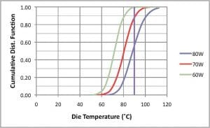
The histograms representing the output of Eqn. 4 in response to the input of the random samplings of ΘJA, power, and ambient temperature values are shown in Figure 5a. Figure 5b depicts the Probability Density Function created by simply plotting the values of the histogram in an x-y plot. The associated Cumulative Distribution Function is plotted in Figure 5c and was created by performing a simple numerical integration in the spreadsheet.
FIGURE 5a. Histogram of calculated distribution of die temperature based on ΘJA distribution and normal distributions of ambient temperature and power and inputting these values into Eqn. 4.
FIGURE 5b. x-y plot based on data in Fig. 5a.
FIGURE 5c. Cumulative Distribution Function obtained by numeri-cal integration of curves in Fig. 5b.
The value at any particular value of junction temperature was generated by adding up all of the values in the distribution to the left of the location to the value at that location. This analysis shows the following percentage of systems that would have a TJ in excess of 90C: 80W, 44.2%; 70W, 13.1%; 60W, 0.6%.
It is useful to compare these findings from applying the Monte Carlo Method to the thermal problem at hand compared with a calculation based on the mean values of all the parameters involved. Plugging the mean values of the parameters into Eqns. 1 – 4 yields a predicted junction temperature of 91.6C at 80W. One might then decide that this 80W value need only be reduced by a few watts to get the maximum value of TJ within acceptable limits. However, based on the Monte Carlo analysis performed here, one sees that making that decision would lead to over 40% of the devices having junction temperatures exceeding the design limit.
CONCLUSIONS
This analysis is intended to demonstrate the mechanics of the Monte Carlo Method in determining allowable power levels for a relatively simple electronics cooling application. However, the method is well capable of scaling to a much higher degree of complexity to deal with situations involving many more design parameters than the situation explored here. Furthermore, the method can readily be adapted to deal with Probability Density Functions other than normal distributions. All that is necessary
is that a suitable function or numerical method be constructed to replicate the experimentally derived distribution. This function would then be used to calculate the Inverse Cumulative Distribution Function that is needed to generate the random sampling of simulated outputs from the thermal model.
REFERENCES
[1] S. Raychaudhuri “Introduction to Monte Carlo Simulation,” Proceedings of the 2008 IEEE Winter Simulation Conference. (Available for download at: http://www.informs-sim. org/wsc08papers/012.pdf)
[2] B. Guenin, “Thermal Interactions Between High-Power Packages and Heat Sinks, Part 1,” ElectronicsCooling, Vol. 16, No. 4, Winter, 2010.”
[3] B. Guenin, “Thermal Interactions Between High-Power Packages and Heat Sinks, Part 2,” ElectronicsCooling, Vol. 17, No. 1, Spring, 2011.
[4] B. Guenin, “Transient Modeling of a High-Power IC Package, Part 2,” ElectronicsCooling, Vol. 18, No. 1, Spring, 2012.”
[5] Wikipedia article, “Normal Distribution” URL = http://en.wikipedia.org/wiki/Normal_distribution
[6] Wikipedia article, “Standard Deviation” URL = http://en.wikipedia.org/wiki/Standard_deviation

