Throughout their careers, engineers and scientists are all likely to encounter and utilize the results of regression analysis, which is “a set of processes for estimating the relationships between a dependent variable and one or more independent variables” [1]. In other words, regression analysis uses a set of data to estimate a relationship between the independent ‘predictor(s)’ and a ‘response’ or ’output’ parameter. In its simplest form, a response, y, may be linearly related to a single predictor, x, in a relationship of y = mx + b. Regression analysis provides a method for estimating values of the constants m (the slope) and b (the intercept).
Regression analysis can be accomplished with different approaches that could include, at least theoretically, a piece of wood, drywall screws, rubber bands and a welding rod1 , as shown in Figure 1. In this regression analysis, screws were put into x-y locations of a graph drawn on the wood and rubber bands between the welding rod and the screws hold the welding rod in an equilibrium position that allow the slope and the intercept to be determined.
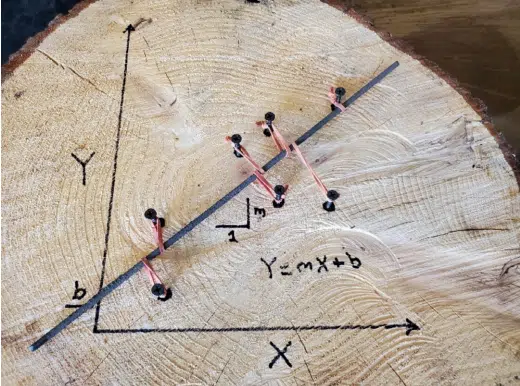
A slightly easier and certainly more accurate approach for conducting a regression analysis is the use of Least Squares. In this approach, rather than the location of the welding rod that leads to a balance in the forces generated by the rubber bands in Figure 1, the ‘welding rod’ corresponds to the straight line that produces the smallest value of E, where E is the sum of squares of the distance in the y-direction between the line and each data point. The equations for calculating the coefficients for a least-squares estimate for linear regression with a single predictor, i.e., y = mx + b, are shown in Equations {1} and {2} [2]:
where xi and yi are the x-y values for the ith data point x̄ and ȳ are the mean values of the x and y data respectively. The coefficient of determination, R2 , is another important parameter in regression analysis. This term describes how well the regression analysis describes the data: an R2 of 1 indicates a perfect fit while a value of 0 indicates that the regression analysis does not predict the response from the input data. R2 is calculated using Equation {3}:
where SSE is known as the sum of squares error.
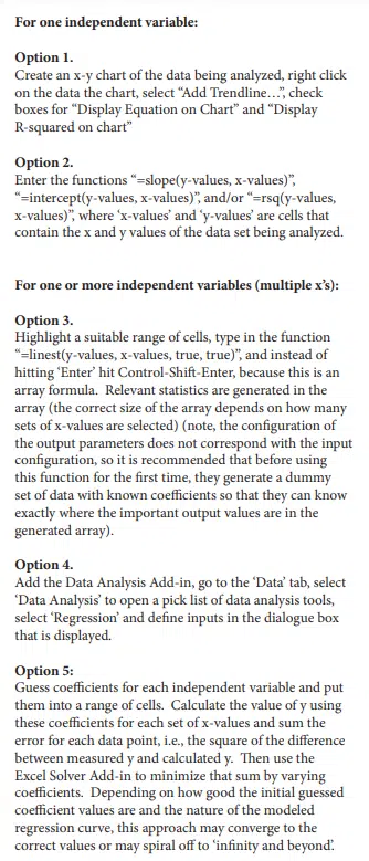
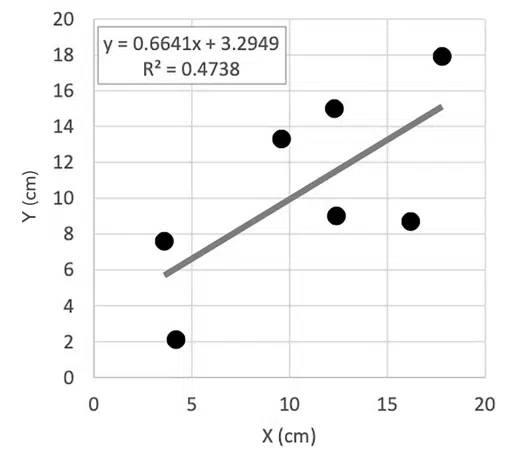
Equations {1-3} are implemented in any software that does regression analysis. For example, several methods can be used in Microsoft Excel to determine regression coefficients. Methods that this author has used are summarized in Figure 2. Figure 3 shows an example of an Excel regression analysis, using Option 1 as described in Figure 2, for the x-y values that were used in the demonstration illustrated in Figure 1.
A previous column in this series described how probability distribution concepts could be used to a confidence interval for a limited set of data. When measurements are used to determine an average value, we can determine what range of values the actual average of the falls within a range to a given confidence level [3]. The confidence interval depends on the variance of the measurements (standard deviation) and the number of measurements made. The t-distribution was used in the calculation of the range.
In the same manner that we estimate a mean value within a confidence interval, confidence intervals also apply to the coefficients (slope and intercept) determined through regression analysis. These intervals are determined with Equations {4} and {5} [2]:
Confidence band on the slope:
Confidence band on the intercept:
Where ta/2 is the t-distribution corresponding to the confidence level and degrees of freedom, n is the number of data points, Σx2 is the sum of all x values, , S = SSE/(n-2) =
.
Another confidence interval of interest is the value of y that is predicted by the regression analysis for any x-value. This confidence interval accounts for the combined effects of the confidence bands associated with the slope and intercept and is shown in Equation {6}.
Confidence band on y-value:
Where A = 0 if we are estimating the confidence band on the average y value for the population tested and A = 1 for an individual item.
Data from the heat sink assessment discussed in [4] will illustrate how these equations are used to determine confidence intervals of regression coefficients. A flat plate heat sink was tested in still air under a range of orientations relative to gravity. Results for ~20W dissipation values for a range of angles are shown in Figure 4, which includes regression analysis results with R2 of ~86%. While this R2 value is reasonable, the suitability of the fit is probably somewhat questionable: the values at the low and high range of measurements are above the fit while those in the middle are below. This is often an indication that the regression analysis may not be capturing the fundamental physics that influence the results.
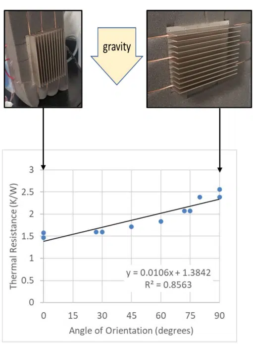
When assessing the results in terms of the physics that cause the heat sink thermal resistance to change with its orientation relative to gravity, it seems reasonable that the buoyant flow that drives natural convection will depend on the cosine of the orientation angle, rather than the angle itself. Figure 5 shows the resulting correlation between the thermal resistance as a function of the cosine of its angle relative to gravity. This appears to improve the fit substantially; the R2 increases from 86% to 95%. Given this improvement in the fit, the subsequent analysis assumes that the cosine of the angle, rather than the angle itself, is the correct independent variable for regression analysis.
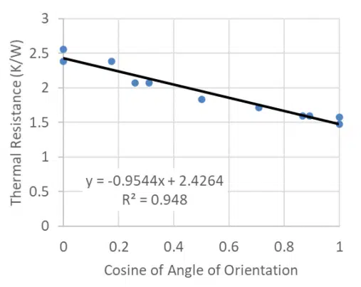
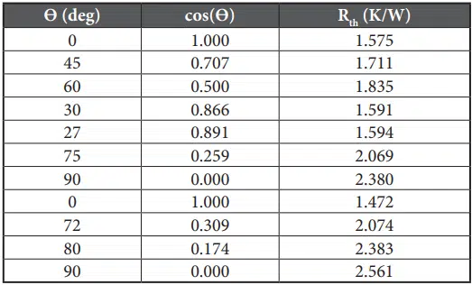
Table 1 shows the eleven data points used to generate the previous plots while the values of the parameters used in, or resulting from, the regression analysis are shown in Table 2 along with brief descriptions of how they are calculated.
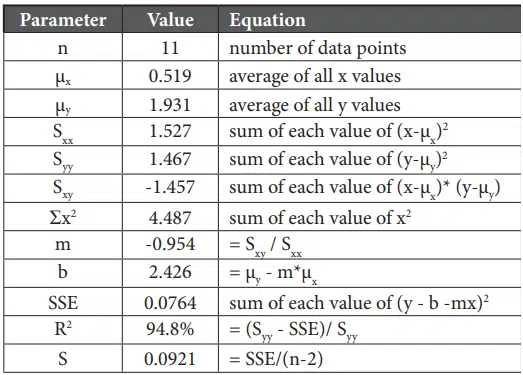
The confidence intervals for the regression coefficients depend on what confidence level is defined. For example, for a 95% confidence level, the t-statistic would be calculated for a probability of 0.975 (1- (1-0.95)/2) and 9 degrees of freedom (sample size of 11 minus 2) as 2.262. The confidence bands for the coefficients are then:
Slope confidence band:
Intercept confidence band:
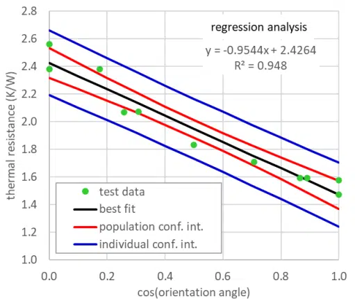
Since the nominal slope and intercept are -0.954 and 2.426, respectively, we can be 95% confident that the slope is between -1.123 and -0.786 (i.e., -0.954±0.169) and the intercept is between 2.317 and 2.536. Using Equation {6}, we can determine the confidence bands for the population and individual measurements, which are plotted in Figure 6.
In summary, conducting a regression analysis can be a relatively straightforward process. Tools are widely available, or the basic equations can easily be implemented into a spreadsheet, to determine a curve fit between independent and dependent variables. One needs to keep in mind, however, that these tools will provide a curve fit, regardless of whether the correct variables have been input to them. As in this case, recognizing the physics of the situation led to a change in the independent variable so that a better fit was obtained. Also, this article described how to calculate confidence bands for the coefficients resulting from a regression analysis, since one must recognize that those values are merely estimates.
References
• https://en.wikipedia.org/wiki/Regression_analysis (accessed 8/7/21)
• J. S. Milton and Jesse Arnold, Introduction to Probability and Statistics: Principles and Applications for Engineering and the Computing Sciences, McGraw-Hill, 1986
• Ross Wilcoxon, “Statistics Corner – Confidence Intervals”, Electronics Cooling Magazine, Spring 2021
• Ross Wilcoxon, “Statistics Corner – Comparing Populations”, Electronics Cooling Magazine, Summer 2021


