The previous articles in this series [1, 2] described how the mean and standard deviations of a set of data are calculated and how they can be used to estimate the characteristics of a population using the normal distribution. Since measured data typically represents only a subset of an entire population, one should recognize that the estimated mean and standard deviation values determined from a sample set are not likely to be exactly equal to the true values of the entire population. In other words, when we calculate the mean, i.e., average, of a data set, we should recognize that there is actually a range of values in which the true population mean lies – and the size of that range depends on the confidence level that we assign to our estimate. This article describes a process that can be used to determine that range as a function of the number of data points and confidence level. More generally, this outlines the overall process for linking probability distributions with confidence levels that is the basis of a variety of statistical analyses.
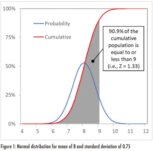
Figure 1 shows an example of a normal distribution in which the mean value is 8 and the standard deviation is 0.75. Two lines are included in this plot: the probability distribution corresponds to the probability of any specific value occurring within the population while the cumulative distribution indicates what portion of the population is less than or equal to a given value1. The cumulative distribution curve is equal to the area under the curve of the probability distribution.
Z-value is defined as the difference of a value from the mean, normalized by the standard deviation. For example, with the mean of 8 and standard deviation of 0.75, a measurement of 9 would have a Z-value of (9-8)/0.75 = 1.33. The cumulative normal distribution for this value is 90.9%2; in other words, 90.9% of the population with a normal distribution would have a Z-value that is less than or equal to 1.33. This is illustrated in Figure 1 as the area under the cumulative probability curve for values of 9 and below.
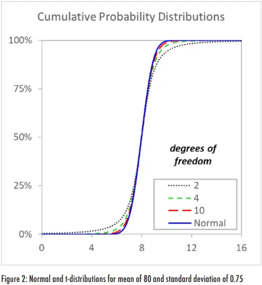
As mentioned previously, we don’t generally know the true mean and standard deviation of an entire population because we only make measurements of a subset of it. The larger the subset (the more samples we use in making our estimates), the more accurate our estimates of the true values should be. When we use a small sample size in an analysis, we can account for the additional uncertainty due to sample size by ‘flattening’ the bell curve of the standard normal distribution and increasing the size of the ‘tails’ (the areas under the curve that are far from the midpoint) using the Student t-distribution.
The t-distribution looks very similar to a normal distribution, but its specific shape depends on the number of degrees of freedom.
The degrees of freedom (DoF) for a sample set corresponds to the number of independent values used in the analysis. In this case, we can consider a data set of n data point to be comprised of n-1 independent values; the difference between the sample size and DoF is due to the use of the data points to estimate the population mean [3]. Thus, one data point is not independent and the other data points can be used to assess to assess the uncertainty. Figure 2 shows t-distributions for 2, 4 and 10 DoF and compares them to the normal distribution, again for a mean of 8 and standard deviation of 0.75. As the DoF increases, the t-distribution converges to the normal distribution; above 30 DoF, the t-distribution is virtually identical to the normal distribution.
With this baseline information on distributions established, we can now describe how they are used to define what range of values the true mean of a population is based on a small number of measurements. The Central Limit Theorem is a critical component in establishing this. The Central Limit Theorem states that a population of terms (X-µ)/(σ/n1/2) tends towards being normally distributed, where X is a value in the population, µ is the mean, σ is the standard deviation and n is the number of samples used to estimate the population characteristics. This applies not only to the data, but also to the distribution that we use to assess our confidence in the mean that is calculated from a sample set.
For example, assume that 50 measurements of a heat sink show that its thermal resistance is 8°C/W with a standard deviation of 0.75°C/W. How confident can we be that the actual population mean is somewhere between 7.9 and 8.1°C/W? Using the Central Limit Theorem, we calculate a test statistic as (7.9-8)/(0.75/501/2) = -0.943. We can look this value up on a standardized normal distribution table, which shows that 17.3% of a normal population that has a mean of 0 and standard deviation of 1 will have a value of -0.943 or less3. Since the normal distribution is symmetric, we will also find that 17.3% of the population will have value of 0.943 or greater. Thus, 34.6% of the normal distribution is either less than 7.9 or greater than 8.1 and there is a confidence band of ~65% that the true mean is between 7.9 and 8.1.
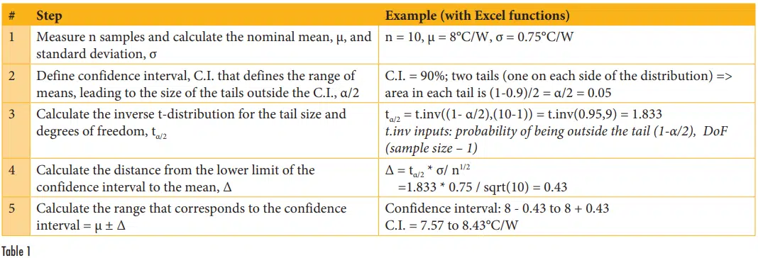
Typically, we are more interested in conducting the reverse analysis – namely, what range of values corresponds to a prescribed confidence band. Also, we may not have the luxury to have a sufficient number of measurements (more than 30) to justify using a standard normal distribution, rather than a t distribution, in our calculations. The steps for determining the range of mean values correspond to a specified confidence band are shown in Table 1. This table includes example calculations for testing on ten heat sinks that again showed a mean thermal resistance of 8°C/W with a standard deviation of 0.75°C/W. The goal of the analysis is to determine the range of values that we can be 90% confident that
the true mean lies within.
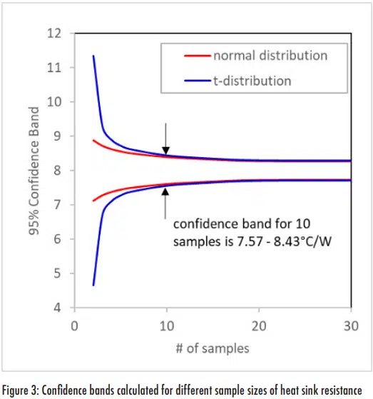
Figure 3 shows the 90% confidence intervals calculated for the tand normal distributions for data with the same mean and standard deviations, but different sample sizes. As the sample size increases, the lines for the confidence intervals come converge. At small sample sizes, the confidence bands that are calculated using the more appropriate t-distribution are much wider than those calculated using the standard normal distribution. In general, it may be questionable that an extremely small sample size of 2-3 samples is necessarily representative of a population – and that small of a sample size also leads to an uncomfortably large confidence interval. But when dealing with typical sample populations with 5-20 measurements, the t-distribution provides a reasonable approach for estimating the confidence interval and can be evaluated for whether it is likely from a normal distribution (a discussion for a future article). When the sample size is greater than 30, the normal distribution can be used to assess the confidence interval. However, since the t-distribution converges to the normal distribution at large sample sizes, one can continue to use the t-distribution even with larger populations. So in general, if these equations are incorporated into a tool such as Excel, it is appropriate to use the t-distribution even for very large sample sizes.
In summary, the goal of the first three articles in this series has been to provide a sufficient background to allow readers to better understand future articles aimed at providing practical statistical analysis approaches. Hopefully, the articles did not achieve a ‘worst of both worlds’ status in which they included more theory than engineers might want to see and less theory than statisticians would expect. Regardless of whether they achieved that or not, with a basic statistical foundation in place we can now move on in future articles to describe tools and analysis methods for solving the types of statistical problems that engineers may encounter.
References
- Ross Wilcoxon, “Statistics Corner—Probability”, Electronics Cooling Magazine, Spring 2020
- Ross Wilcoxon, “Normal Distribution”, Electronics Cooling Magazine, Summer 2020
- https://blog.minitab.com/blog/statistics-and-quality-data-analysis/what-are-degrees-of-freedom in-statistics


