Introduction
The previous column in this series described methods for assessing whether a set of data was normally distributed [1]. In the event that data is shown to not have a normal distribution, one might ask how to conduct a statistical analysis on it given that many statistical tests are developed on the assumption that the data are normal. For example, how can two non-normal data sets be analyzed to determine whether one is statistically better than the other?
Nonparametric statistics are used to analyze data that are not well described by discrete parameters, such as the mean and standard deviation used to describe a normal distribution. One useful method in nonparametric statistics is the Wilcoxon Rank Sum (WRS) Test, which is also known as the Mann-Whitney-Wilcoxon test. The WRS test analyzes the ranks of an ordered data set rather than the direct values of actual values. This is analogous to how the median may provide a more representative assessment of a population than the mean, if the data set includes a few extreme values (such as in determining the typical net worth of a small group of people that happens to include a billionaire).
Rank Sum Test Procedure
The WRS test procedure begins by combining two data sets and sorting them in order of lowest to highest values (sorting from highest to lowest also works). The ranks of each value in the sorted values for each data set are then added together. In the event that two or more values have the same rank, then they are all assigned the same average rank.
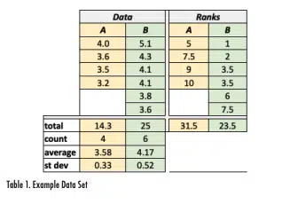
Consider the two data sets (A and B) shown in Table 1, which includes a total of ten measurements (4 in Data Set A and 6 in Data Set B). The largest term in the combined list of data is the value of 5.1 in Data Set B, so it has a rank of 1 (as shown in the column on the right edge of the figure). Data Set A includes the smallest measurement of 3.2, which corresponds to the 10th rank in the combined data set. Data Set B includes two values of 4.1, which ranks 3rd in the combined list. Since these two would occupy ranks 3 and 4 in the list, they are each assigned the average rank of 3.5.
Once the rank for each data value has been assigned, the ranks are added together. For example, the ranks for Data Set A are 7.5+5+10+9=31.5 and the rank sum for Data Set B is 23.5. The rank sum value for the data set with the smallest number of terms is then compared to the WSR critical values for a given probability value.
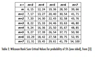
Table 2 shows a set of WRS critical values for a 5% one-sided distribution (and 10% two-sided distribution for values of m and n, where m is the number of values in the data set with the fewest terms and n is the number of terms in the other data set.
For the case corresponding to the data in Table 1, the critical values for m=4 and n=m+2=6 are found in Table 2 to be 14 and 30. The rank sum for Data Set A was calculated as 31.5, which is outside the range of 14-30. Therefore, one can conclude to a 90% confidence level that Data Set A is different from Data Set B, i.e., that the higher values of Data Set B relative to Data Set A is statistically significant.
Note that if the data were analyzed using a conventional t-test, the same conclusion with a similar confidence level would be found.
How WRS Critical Values are Found
Since nonparametric tests like the WRS test are not dependent on assumptions regarding the distribution and are less influenced by individual outlier data points, one might ask why the WRS test is not always used instead of a test such as the t-test. One likely reason is that there is no direct method for determining the WRS test critical values. Typically, those values are found from a table such as that shown in Table 2 or more extensive tables such as Reference [4]. Readers who are content with simply using terms listed in a critical value table, may choose to skip the rest of this section. Those readers who, like this author, are bothered by ‘magically appearing’ terms and want to better understand how the critical values are generated, may choose to read on.
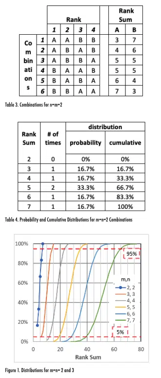
The WRS critical values are generated by determining the rank sums that could result from every combination of a data set with a given size. For example, consider two data sets for A and B where each set only includes 2 values. The number of possible combinations of ranks that could be generated is found with the ‘n choose k’ formula that determines how many combinations of k terms can be generated with n variables. With this equation, the number of possible combinations of ranks is (n+m)!/(n!*m!), so for the case of n=m=2, the number of combinations is (1*2*3*4)/(1*2)/ (1*2) = 6. These six possible combinations are shown in Table 3; for Combination 1, for example, the two highest largest terms are from set A and the smallest two terms are from set B. This table also shows the rank sums for each combination for the two data sets.
Table 4 shows the probability and cumulative distributions of each rank sum, which are the number of occurrences equal to and less than or equal to that rank sum, respectively, divided by the number of combinations.
Figure 1 plots the values shown in the last column on Table 4 for m=n=2 (with symbols and a line) as well as lines that show the cumulative distributions for m=n=3, 4, 5, 6, and 7. The figure also includes horizontal lines for cumulative probabilities of 5% and 95%. The intersections of these horizontal lines with the cumulative distributions correspond to the WRS critical values. For example, the m=n=7 distribution intercepts the 5% and 95% lines at Rank Sum values of approximately 40 and 65, respectively. Those values agree well with the terms shown in Table 2 of 39 and 66 (in the upper right-hand cell of the table).
While the process of calculating the WRS critical values is straightforward, it can be computationally intensive. To calculate the critical values for m=n=7, for example, includes accounting for 14!/(7!*7!) = 3432 combinations. Doubling the number of terms to m=n=14 increases the number of combinations to evaluate to more than 40 million.
As the number of data points increase, the WRS distributions more closely approximate a normal distribution. The differences between the distributions become increasingly isolated to the extreme tails.
Summary
Data may not always be easily characterized with a parametric distribution such as the normal distribution. In those cases, nonparametric tests like the Wilcoxon Rank Sum test may be used. This test can serve a similar role as the t-test, but uses the ranks of terms in the combined data set, similar to a median value, rather than average and standard deviations of data sets.
Because there is no direct method for calculating the critical values for the WRS test, it is typical that these values are found in a table. As the size of the samples increases, the WRS distributions used to calculate the critical values more closely approximate a normal distribution. Therefore, when the total number of samples gets larger than ~20-30, the impact of using the WRS test or assuming a normal distribution will likely become negligible. In those cases, it may become important to identify outliers that have an excessive influence the results. This is the topic of the next article in this series.
References
[1] Previous statistics corner
[2] https://en.wikipedia.org/wiki/Frank_Wilcoxon
[3] Milton & Arnold, “Probability and Statistics in the Engineering and Computing Sciences, McGraw-Hill, Inc., 1986
[4] https://users.stat.ufl.edu/~winner/tables/wilcoxonmannwhitney%5B1%5D.pdf


