Normal Distribution

Introduction

The previous column in this series [1] discussed statistical probability and showed that the plot of the probability of a given value occurring within a population can look like a hill in which there is a peak in the middle that tapers off to increasingly smaller slopes on each side. The example in that column referred to the scores produced by shaking a number of dice, and the ‘hilly’ plot was described with the more common term of ‘bell-shaped curve’. The purpose of establishing a probability distribution to describe a population of data with uncertainty is that it provides a mathematical framework for dealing with that uncertainty—if a reasonable mathematical model of the distribution curve can be defined. As we will see in subsequent columns, many different models for probability distributions exist; the selection of the correct model depends on characteristics of the population and what data are available for analysis.

This column focuses on the probability model that is most widely used and most recognized: the Gaussian, or normal, distribution. The normal distribution, as written in terms of a probability density function is shown in Equation (1):

(1)

Equation (1) allows one to estimate the probability of a given value, x, occurring in a population that is defined with the two parameters μ and σ. While the normal distribution equation itself may not be familiar to everyone, the terms μ and σ should be recognizable to anyone who deals with data: μ is the mean (or average) value and σ is the standard deviation. If the mean and standard deviation of a population are known, the probability that a randomly selected member of that population will have a value of x can be calculated with Equation (1). Or, if you are like me and rely on spreadsheets to do most of your calculations, you can use the function: @norm.dist(x, μ, σ, false).¹

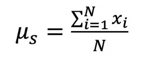
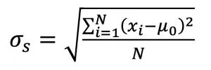
The mean and standard deviations can be calculated for a set of N samples, x₁, x₂, …x_n, by:

(2)

(3)

Equations (2) and (3) include the subscript ‘s’ for the mean and standard deviation as a reminder that the values determined from a sample (the set of data drawn from a population) are not exactly equal to those for the entire population (all possible elements). Traditionally, the mean and statistical deviation of a sample are written as x and s, respectively. A future column in this series will discuss how to use the values of μ_s and σ_s, also known as x and s, to determine a range in which we can be confident that the population mean, μ, actually lies. Note that the mean and standard deviation of a data set can be calculated in a spreadsheet with the functions @average(‘data’) and @stdev(‘data’), respectively, where ‘data’ refers to the cells that contain the data.

Our familiarity with the term ‘average’ can lead to its occasional misuse, which can be avoided if we keep its relationship to the normal distribution in mind. The version of the classic illustration of a misuse of the term ‘average’ is the example of nine people, who all have a net worth of $500,000, are sitting in a bar. In walks the founder of a “multinational conglomerate technology company that focuses on e-commerce, cloud computing, digital streaming, and artificial intelligence” who has a net worth of $140B. Using Equation (2), the average net worth of the individuals in the bar suddenly increases to $14B, which may be mathematically correct but not physically relevant. The primary basis for this discrepancy is the fact that the population of the 10 individuals in the bar is not representative of a normal distribution. In cases like this, the median may be a more appropriate parameter for reporting a typical value. The median is the middle value in a ranked list of the sample set such that an equal number of values are greater than and less than it (the spreadsheet function for calculating median is @median(‘data’). When the mean and median of a data set are substantially different, such as in the aforementioned example of the people in the bar, one should suspect that the sample set is not normally distributed.

A fundamental strength and justification for utilizing the normal distribution is the central limit theorem, which shows that when multiple, independent random variables are added, the result tends towards a normal distribution—even if the variables themselves are not normally distributed (see for example Reference [2]). Reference [1] discussed the results of throwing dice, beginning with the assumption that a single die is ‘fair’ such that the probability of it showing any particular value is equal to the inverse of the number of sides on the die (i.e., 1/6th for a six-sided die). The distribution of scores that result from throwing that one die is certainly not normal; it would be a straight line with equal probability of 16.7% for each of the six values. With two dice, the distribution had a triangular shape and, as the number of dice increased, the distribution looked more and more like a bell-shaped curve.

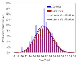
Figure 1 shows simulated results for throwing 6 six-sided dice 100 and 5,000 times. The larger number of throws leads to a more well-behaved distribution of results (red bars appear to be more ‘bell shaped’). However, both data sets produce very similar normal distributions with mean values of ~21 and standard deviations of 4.2. This illustrates the power of the normal distribution and the results of the central limit theorem. Even when we have results from a small data set that in of itself does not appear to be normally distributed (have a ‘clean’ bell-shaped curve), if the data were drawn from a normal distribution there is a good chance that they can be used to accurately estimate the fundamental characteristics of that population.

The normal distribution provides a straightforward method for using measurable characteristics of a data set (the mean and standard deviation of the sample) to estimate the probabilities of future measurements falling within a prescribed range of values (related to the properties of the entire population). This is incredibly useful in that it allows us to perform tasks such as:

• Determining how many samples must be measured to have confidence that a population has been adequately characterized
• Comparing different data sets and decide with they are from the same population or not (e.g. to determine if differences in their mean values are ‘statistically significant’)
• Deciding whether a value that seems to be an outlier is likely to be from the population that we are evaluating or if it is due to a factor such as a measurement error,
• Defining how much confidence we should have in a curve fit we generate from a data set

These types of practical tools are all topics that will be discussed in future columns, now that these foundational topics of probability and distributions have been covered.

¹ The ‘false’ in this equation specifies that the probability distribution (a bell-shaped curve that goes to zero as x goes to infinity) is calculated. If ‘true’ is used instead, the function returns the cumulative distribution (an S-shaped curve that goes to 1 as x goes to infinity)

² Equation (2) defines the arithmetic mean, which is the same as the arithmetic average. The more generic terms mean and average are often used interchangeably but can refer to different definitions.

References

1. Ross Wilcoxon, “Statistics Corner—Probability”, Electronics Cooling Magazine, Spring 2020, pp. 16-18
2. http://sphweb.bumc.bu.edu/otlt/MPH-Modules/BS/BS704_Probability/BS704_Probability12.html