Introduction
Previous articles in this series described the normal distribution and how it is used to relate probability and confidence levels [1, 2]. A practical application of the use of the confidence interval was to describe how to determine the range of values in which the true mean of a population falls within, based on the mean and standard deviation calculated from a set of samples drawn from the population. This range depends on the confidence level that is selected for the analysis and the number of samples used to estimate the population. The fewer samples or the higher the confidence level that is selected, the wider the range in which the true mean value may lie.
This article discusses how the confidence band concept is extended to compare different sample sets to determine, within a set confidence level, whether the two sample sets have the same mean. This provides a statistically established method to determine if two data sets are different, thereby demonstrating whether a treatment, design change, etc., lead to an improvement.
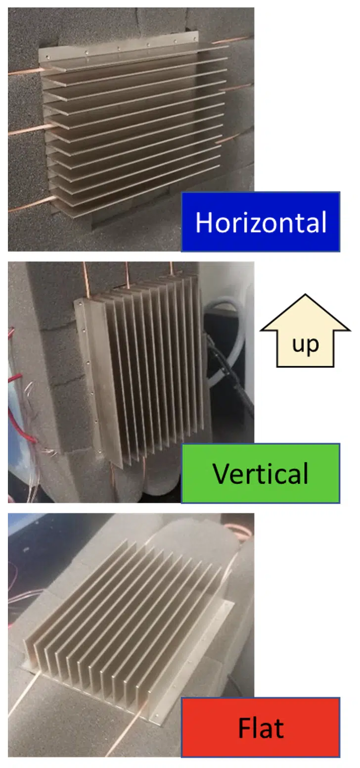
Figure 1. Heat sink orientations for natural convection testing
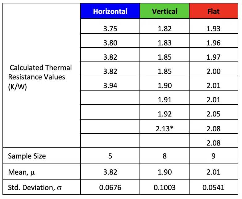
The following example illustrates the overall procedure for comparing two populations to determine whether they are different. Somewhat rudimentary testing1 was used to evaluate a natural convection heat sink in the three different orientations illustrated in Figure 1. In the Horizontal orientation, the base of the heat sink was aligned with the direction of gravity and the fins were perpendicular to gravity. In the Vertical orientation, the heat sink base was again aligned with gravity, but the heat sink was rotated 90° such that the fins were parallel to gravity. In the Flat orientation, the fins faced upwards with the base perpendicular to the direction of gravity. Table 1 shows individual thermal resistances calculated from different tests and calculated values for the number of data points (n), mean (μ), and standard deviation (σ) for each heat sink orientation. In this testing, power was dissipated from a heater attached to the back of the heat sink. The average heat sink temperature was determined with four thermocouples attached to the heat sink and the thermal resistances were calculated by dividing the temperature difference (average heat sink temperature minus ambient air temperature) by the heater power dissipation. Tests were repeated over a number of days with different heater powers and with the orientations relative to gravity randomized. Testing did not control for the effects of radiation, minor room drafts, heat losses from the back of the heat sink, etc. Therefore, the data shown in Table 1 are primarily useful for comparing the effects of orientation, and do not represent a controlled investigation to determine the precise heat sink resistances. While testing was conducted over a broad range of power dissipations, the data in Table 1 are limited to rest data for power dissipation in the range of 20-25W.
Table 1. Heat sink thermal resistance test data
Based on the sample mean values of the thermal resistances, it appears that the Horizontal orientation has a significantly higher thermal resistance (of 3.82 K/W) than the Vertical orientation (resistance of 1.88 K/W) and the Flat orientation (2.01 K/W). The questions that we will attempt to answer in this analysis are 1) what is our confidence that the Horizontal thermal resistance is actually different from the other orientations and 2) is there a statistically significant difference in the thermal resistances of the Vertical and Flat heat sink orientations?
Using the procedure described in [2], we can use the calculated mean, standard deviation and sample size to determine the range in which the true mean lies, for a given confidence level, of each set of measurements. With fewer than 30 measurements, we assume that they follow a student t-distribution, which is defined as a function of the confidence level and number of degrees of freedom (d.f.), which is equal to n-1 for a single set of measurements. Values of the t-distribution can be found in tables in any statistics text, many online resources such as [3], or software such as Excel. Again, as shown in [2], the range in which the true mean (μtrue) of a population is lies is calculated as a function of the measured mean (μmeasured),
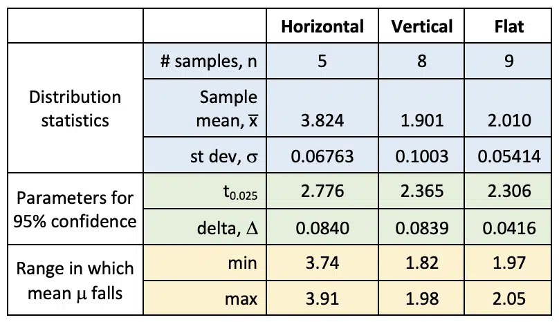
For example, with the horizontal data, in which 5 measurements produced an average of 3.82 and standard deviation of 0.676, we can be 95% confident that the true mean falls between 3.74 and 3.91 2. The parameters used to calculate the confidence intervals and the ranges for the 95% confidence interval for the mean thermal resistance for each of the three heat sink orientations are shown in Table 2. This table includes each value of t corresponding to the degrees of freedom (sample size – 1) and the confidence level of 0.025, which is calculated by (1 – 0.95)/2 with the 2 corresponding to a two-tailed distribution.
Table 2. Terms used to determine 95% confidence intervals for thermal resistance of each orientation
The results in Table 2 indicate that we can be more than 95% confident that the thermal resistance of the heat sink in the Horizontal orientation is higher than in the other two orientations, since there is no overlap between its range and the others (3.74 is greater than both 1.98 and 2.05). However this approach using a 95% confidence level, indicates the Vertical and Flat thermal resistances are not statistically different since there is a slight overlap in their ranges (1.97 falls between 1.82 and 1.98).
This analysis can be improved by recognizing that the size of the range for a given confidence level is due to a combination of the standard deviations and the number of samples of each test set. Even if the means of two populations are different, their standard deviations may be similar enough that we can ‘pool’ the data and increase the effective sample size by accounting for the number of samples in each data set.
We can use the F-distribution to determine whether we can pool data to increase the effective sample size. Without going into the detail that it deserves, the F-distribution is a statistical distribution that can tell us the probability that the variances, i.e., standard deviations, of two populations are different – in a similar manner that the t-distribution indicates the probability that the means of two populations are different. We can use the Excel function @f.test(array1, array2) to determine whether the standard deviations of two populations are different, and therefore that data can be pooled to determine the confidence range for the mean. The arrays in that function are the two sets of measurements under consideration and the function returns the probability that the standard deviations are different.
In comparing the Vertical and Flat data, the F-test function returns a value of 10.5%. Since this is greater than 5%, we cannot conclude (at a 95% confidence level) that the variances (standard deviations) of the two populations are different. Therefore, we can pool the data in applying the t-test that determines whether the means of the two population are different. The pooled standard deviation, σp, can be calculated using the estimated standard deviations (σ) and sample sizes (n) of each sample set, as shown in Equation 2 [3].
The pooled standard deviation of the Vertical and Flat data is calculated to be 0.006262. This is then used to calculate the test statistic, T, for the pooled data, which is determined with Equation 3:
For the pooled Vertical and Flat data, this is calculated to be 2.8259. This value is then compared to the t-value that is calculated for the selected confidence level and the total degrees of freedom, which is the sum of the samples from the two data sets minus 2 (since one degree of freedom was ‘consumed’ in calculating each of the two means). For a 95% confidence level and a two tailed distribution, the input parameter for the t-test is α/2 = (1-0.95)/2 = 0.025. In Excel, a value of α/2 that is less the 0.5 will return a negative number, so the t-value for the pooled sample can be calculated with =-t.inv(0.025,(8+9-2)) = 2.13144 3. Since this value is less than the test statistic of 2.8259, we can be 95% confident that average thermal resistance for the Vertical heat sink is different from the Flat heat sink. If we repeat the analysis with a confidence level of 98.72%, the t-statistic is equal to the T-value of 2.8259. If one prefers to type in fewer equations, a simpler approach to reach the same conclusion is to use the function =1 – t.test(array1, array2, 2, 2), where the two arrays are the two sets of data for the Vertical and Flat orientations. In this function, the first 2 indicates that the distribution is two-tailed, and the second 2 indicates that the two data sets are homoscedastic (with the same variance, as determined by the F-test). This function, with the two sets of data returns a value of 0.9872; since this value is larger than 95%, we can conclude with a 95% confidence level that the thermal resistances for the Flat and Vertical orientations are different.
If the F-test finds that the variance of the data sets ae unequal, the Smith-Satterthwaite procedure [3] can be used to estimate an effective number of degrees of freedom in the pooled data (npooled) using Equation 4:
where the function rounddown<> rounds the result down to the integer value.
Summary
The t-test provides a method for estimating a range that we can be confident that a population mean falls within, based on a limited sample size. This article described how that can be extended to compare two data sets to determine whether the populations have different mean values. The F-test provides a similar method for determining whether the variances of two populations are the same in order to justify whether two data set can be pooled together to increase the effective sample size and thereby increase the confidence of conclusions.
Author Notes
1. Readers with a reasonable background in statistics may have noticed that I am often a bit careless in my treatment of the mean and standard deviation of a population/sample. A rigorous approach would differentiate between quantities relevant for the complete population (the true mean and standard deviation) compared to the estimated values based on the subset of the population that is sampled. The goal of these article is to provide reasonably simple tools for drawing statistical conclusions without diving too far into the statistical details. I hope that my attempts to minimize confusion that can be generated by additional notations and parameters do not actually increase confusion due to a lack of sufficient context.
2. I slightly modified the data set in order to better demonstrate the impact of pooling data sets. The highest thermal resistance value for the Vertical orientation (2.13, which is indicated with an asterisk) was actually measured to be 1.93 in testing. It is left to the interested reader to calculate how the use of the correct value affects the overall confidence level.
1 Note the rubber bands and packing foam used in the test setup
2Calculation method: n = 5, μ = 3.824, σ = 0.06763, d.f. = n-1 = 4. 95% confidence for two tailed distribution => α/2 = (1-0/95)/2 = 0.025; t-statistic in Excel is t0.025 = abs(t.inv(α/2, d.f.) = abs(t.inv(0.025, 4) = 2.7764 ∆ = t0.025*σ/n1/2 = 2.7764*0.06763/51/2 = 0.084, mean range = μ ± ∆ = 3.824 – 0.084 to 3.824 + 0.084 = 3.74 to 3.91
3Alternatively, Excel will also return the correct positive value if we use 1-α/2: =t.inv(0.975,15) = 2.13144.
References
1. Ross Wilcoxon, “Statistics Corner – Normal Distribution”, Electronics Cooling Magazine, Summer 2020, pp. 10-11
2. Ross Wilcoxon, “Statistics Corner – Confidence Intervals”, Electronics Cooling Magazine, Spring 2021, pp. 10-12
3. https://www.tdistributiontable.com/ (accessed May 20, 2021)
4. J. S. Milton and Jesse Arnold, Introduction to Probability and Statistics: Principles and Applications for Engineering and the Computing Sciences, McGraw-Hill, 1986, pp. 297-308


