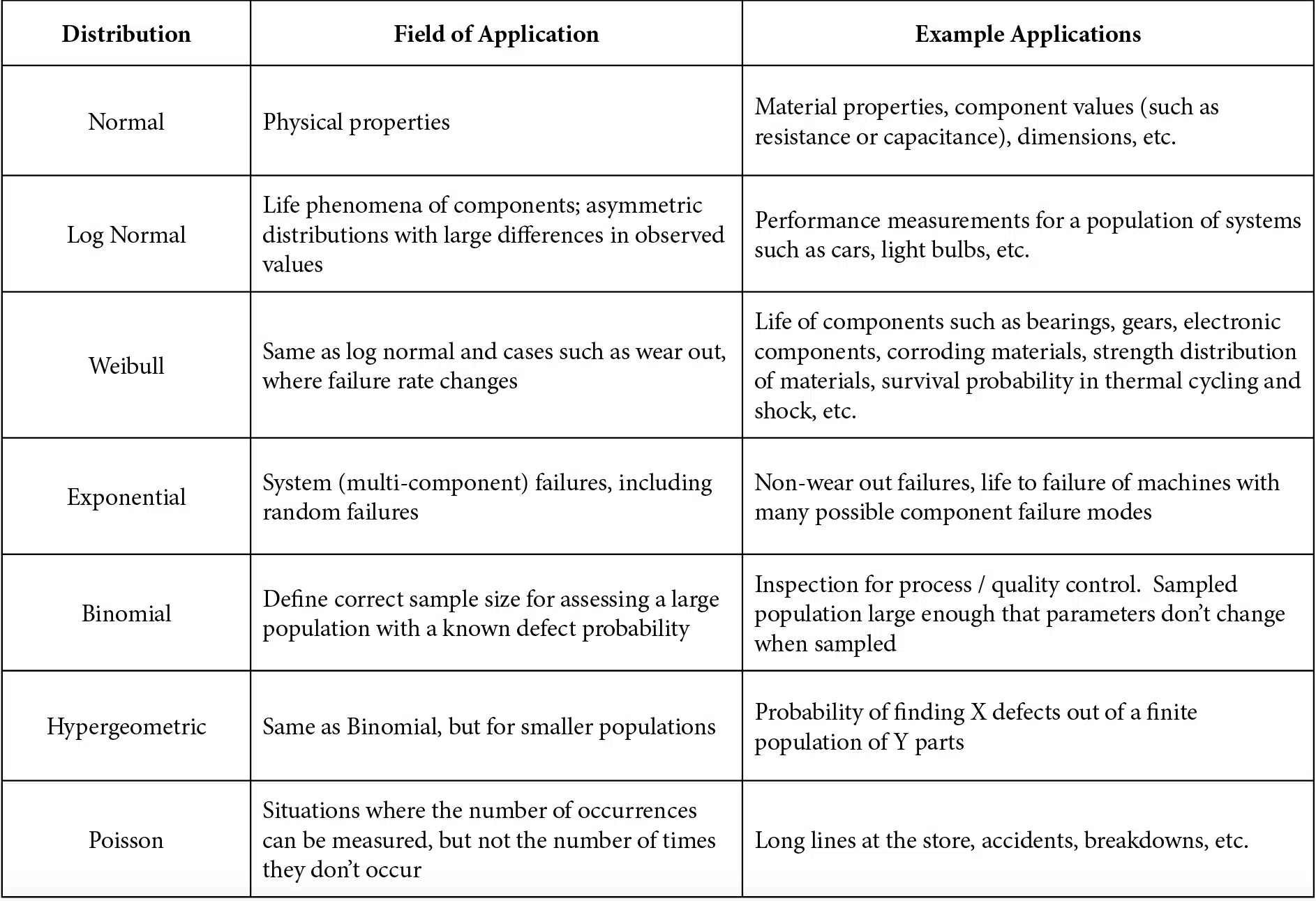
A little over a pandemic ago, the first article in this series on statistical analysis mentioned that a fundamental aspect of statistics is that one assumes a mathematical model that describes the distribution of a data set and then uses that model to estimate the probability that a given value or set of values will occur [1]. This allows us, for example, to estimate whether two sets of data are from the same underlying population or if they are statistically different. The statistical analyses discussed thus far have primarily assumed that a population has a normal distribution. However, there certainly are other distributions that can, and should, be used for different types of data. Table 1 lists a few common statistical distributions with brief descriptions and examples of how they are applied.
Table 1 Common statistical distributions (adapted from Table 2.2 of Ref. [2])
Lognormal and Weibull distributions are often applied to analyze reliability data for situations such as the wear out of solder joints that have been subjected to multiple thermal cycles. As a reminder, the formula for the probability of a given value of x in a normal distribution is shown in Equation {1a}. The mean, m, and standard deviation, s, for a population x can be easily calculated. Therefore, the probability distribution, f(x), of the normal distribution can be calculated directly with Equation {1a}. The cumulative distribution, F(x), which is the area under the probability distribution curve to the left of a value x, is found by integrating the probability distribution, as shown in Equation {1b}.
The lognormal distribution is also calculated using Equations {1}, except that the values of x that are used to calculate m, s, and f are all the natural logs of the population values.
The Weibull distribution is defined such that its cumulative distribution1 is calculated as shown in Equation {2}.
As with the probability distribution of the normal distribution, the cumulative Weibull distribution can be directly calculated for any value of x once the two terms that characterize the distribution are known. Instead of the mean and standard deviation used in the normal distribution, the Weibull distribution uses the characteristic life (also known as the scale parameter), q, and the shape parameter, b. Physically, these two terms are similar to their normal distribution counterparts: the characteristic life is analogous to the mean, but instead of indicating the 50% failure point (for failure data), q corresponds to the point at which 63.2% (1-1/e) of the population would fail. Because of this, the characteristic life is often referred to as N63. The shape parameter, b, also known as the Weibull slope, is analogous to the inverse of the standard deviation. The larger the shape factor, the smaller the spread in the data.
While the Weibull coefficients (q and b) are physically analogous to the normal distribution coefficients (m and s), there are no formulas for directly calculating the Weibull terms as there are with the normal distribution terms. The Weibull coefficients can be calculated using a different approach that is ultimately at least part of the reason that the Weibull distribution has been widely used for analyzing reliability data.
The approach for determining the Weibull coefficients begins by first rearranging Equation {2}, as shown below.
Taking the natural log of both sides of the equation twice gives us:
This can be written as:
This produces a linear equation of the form , where the terms for Y, X, and C are:
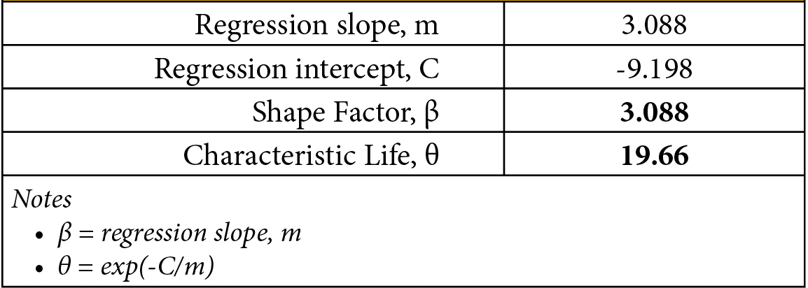
Once the regression analysis has determined the linear coefficients m and C, they can be used to determine the Weibull coefficients. The shape factor is equal to the slope of the regression analysis (b = m) and the characteristic life is determined by rearranging the above equation for C as θ = exp(-C/m).
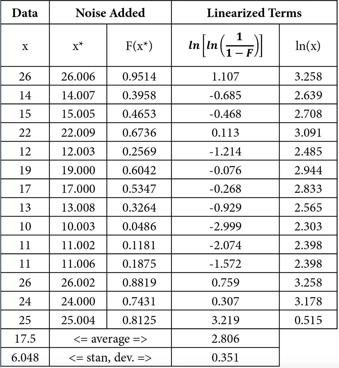
One easy way to generate a set of fatigue data is to count the number of times paper clips can be bent from 0° to 90°, as shown in Figure 1, before breaking. Data for the number of bends needed to break fourteen paper clips are shown in the first column of Table 2. As discussed later, this table also includes processed data used to calculate the Weibull coefficients. As shown in the bottom of the table, the measurements had an average of 17.5 bends with a standard deviation of 6.048.
Figure 1 Paper clip fatigue test configurations
One possible way to define the cumulative failure distribution, F(x), would be to divide the rank of the failure by the total number of samples. For example, if 10 components are tested, the first failure would have F(x) = 0.1, the second one would be 0.2, etc. This approach, however ‘pushes’ F to higher values; for example, only the first failure would be categorized to the lowest 10% while the last two failures would be categorized to the highest 10%. A better approach for calculating the values of F(x) is to use the median ranks, which are typically calculated with Equation {3} [2]
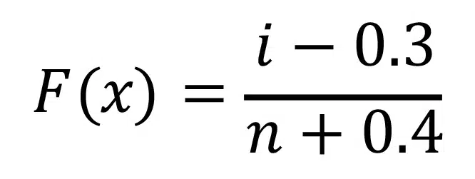
In this equation, i is the rank of the failure and n is the total number of samples. For example, if 10 samples are tested, the first failure would have F(x) = (1-0.3)/(10+0.4) = 0.0673, the second failure would have F(x) = (2-0.3)/10.4 = 0.163, etc.
Since the calculation of F(x) requires that the order of failures be determined (first, second, etc.), the Excel @rank() function can be used to determine the order of failures2. Because of the way that this function deals with ties (each tie has the same rank), a small amount of ‘noise’ was added to the data to prevent any ties when calculating the ranks used for F(x). This noise was generated using the random function, which generates a random number between 0 and 1, by adding the term ‘rand()/100’ to the measured data, x, to create x*. The x* value was only used to determine the rank, which was then implemented in Equation 3 to calculate F(x).
Table 2 Paper clip failures: raw and processed data
Once values of x and F(x) were determined, the linearized data of Y = ln(ln(1/(1-F) and X =ln(x) were calculated. Regression coefficients were determined using Excel functions m=slope(Y,X) and C=intercept(Y,X), as discussed in [3]. Table 3 shows the values determined for m and C as well as the Weibull coefficients determined from them.
Table 3 Regression and resulting Weibull coefficients
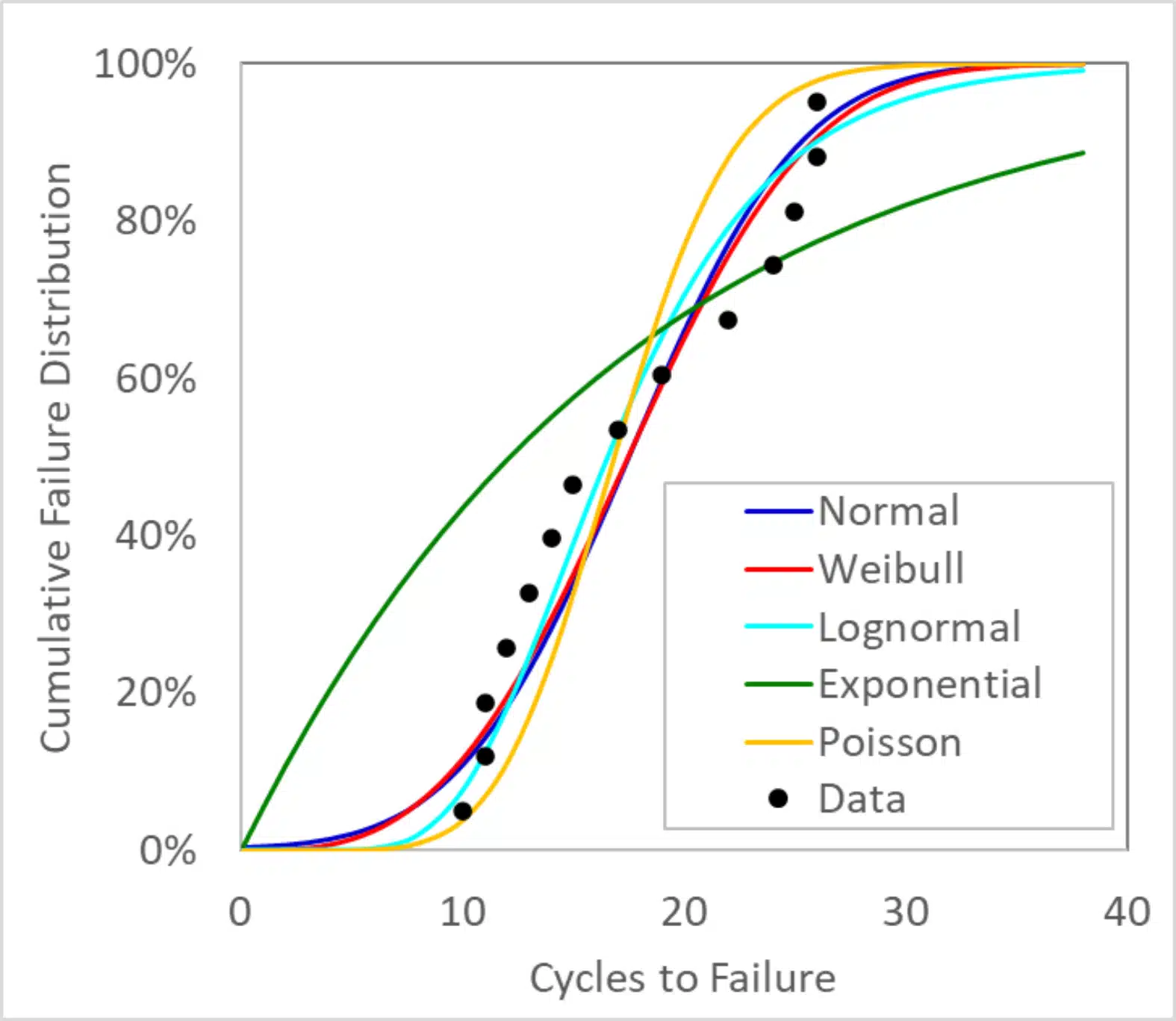
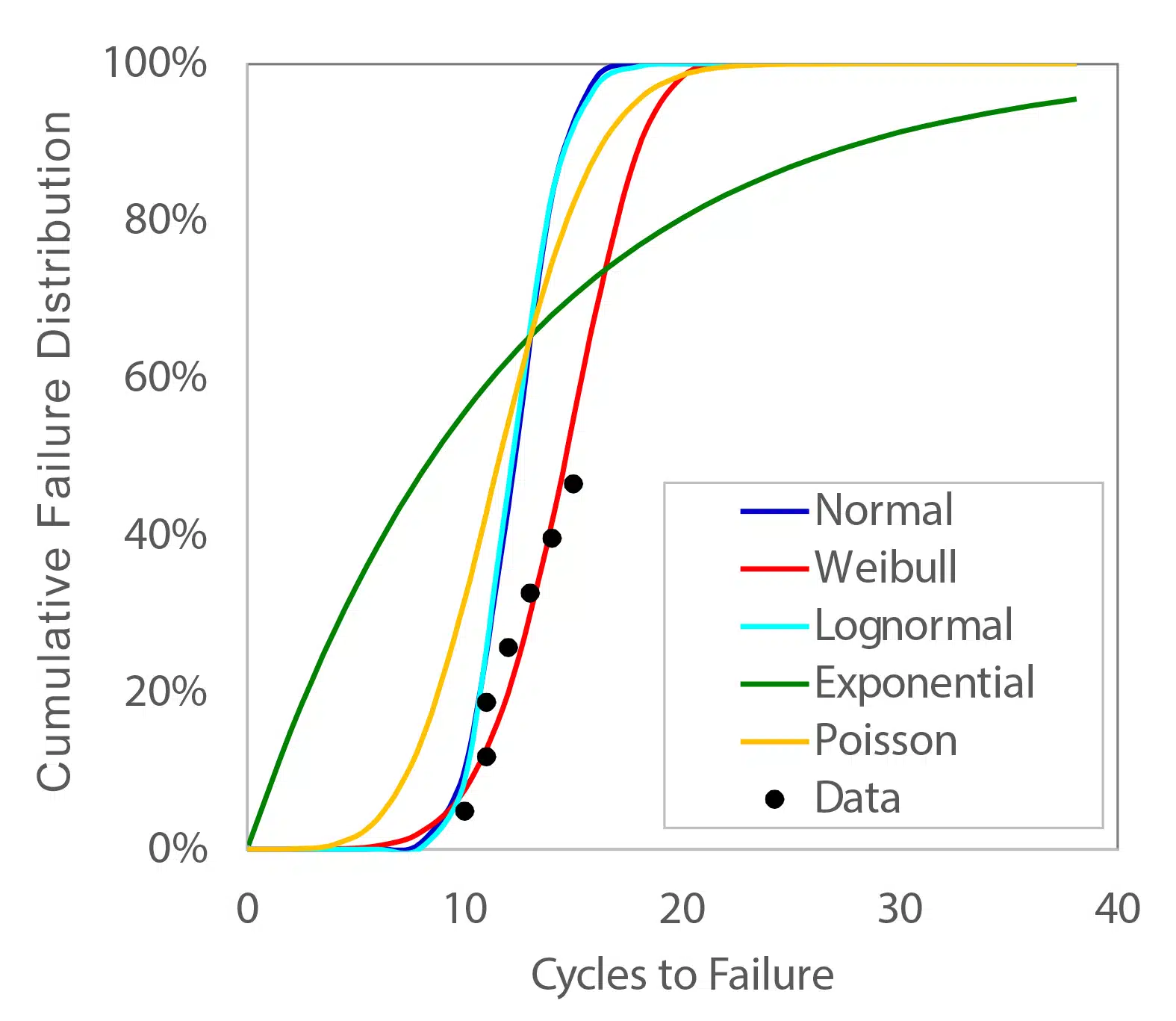
Figure 2 plots the paper clip data along with corresponding fits of the data using many of the distributions listed in Table 1. The Excel equations used to generate these curves are shown in Table 4.
Figure 2 Paper clip data fit to different statistical distributions
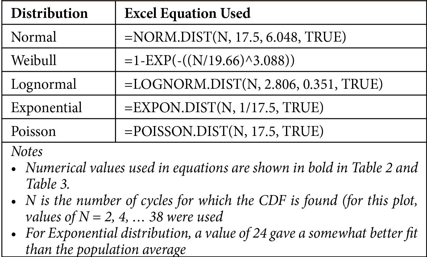
Table 4 Excel functions used to calculate statistical distributions in Figure 2
An interesting observation from Figure 2 is that, except for the Exponential distribution, all of the distributions provided a reasonably good fit to the measured data. The primary differences between the different distributions are in the tails and the knees (where F(x) ~0-10% and ~90-100%). One may then ask then, if the normal distribution, which is used almost everywhere, produces similar results to the Weibull distribution, why is Weibull primarily used for reliability analysis?
One reason is that Weibull distributions, as well as the other non-normal distributions shown, have a physically accurate limit. In those distributions, by definition, F(0) is equal to zero3. In contrast, a normal distribution of failure data includes some portion of the population supposedly failing at negative cycles. This is typically a small value – for the data in Table 2, the normal distribution calculates that 0.318% of the paper clips would fail before the first bend.
The much more important reason why the Weibull distribution has been used for assessing certain types of data, such as that from reliability testing, is that it does not rely on complete knowledge of the entire test population. If an entire set of samples is tested until all fail, the normal distribution – or better yet the lognormal distribution, which passes through F(0) = 0, will likely describe the data as well as the Weibull. However, due to constraints in time, budget, testing availability, etc., testing may stop before all samples have failed. If one characterizes the population only using that fraction of parts that have failed, the calculated average life will be much smaller since those components with longer lives would not be included in the calculations.
For example, if the paper clip testing had been stopped after a maximum of 15 bends, only half of the samples would have registered a failure. The average life of those parts would be 12.3 cycles, rather than the 17.5 that was found with the entire population.
Figure 3 Failure distributions calculated only using failures up to 15 cycles
Figure 3 plots the same distributions as were shown in Figure 2, but with truncated data that only included those failures that occurred within 15 cycles. It is not surprising that those distributions that depend on the mean values, which were lower in the truncated data, are pushed to the left and provide a less accurate description of the population of the entire data set. Because the Weibull distribution uses regression analysis of the failures as part of the entire test population, it continues to agree with the actual data.
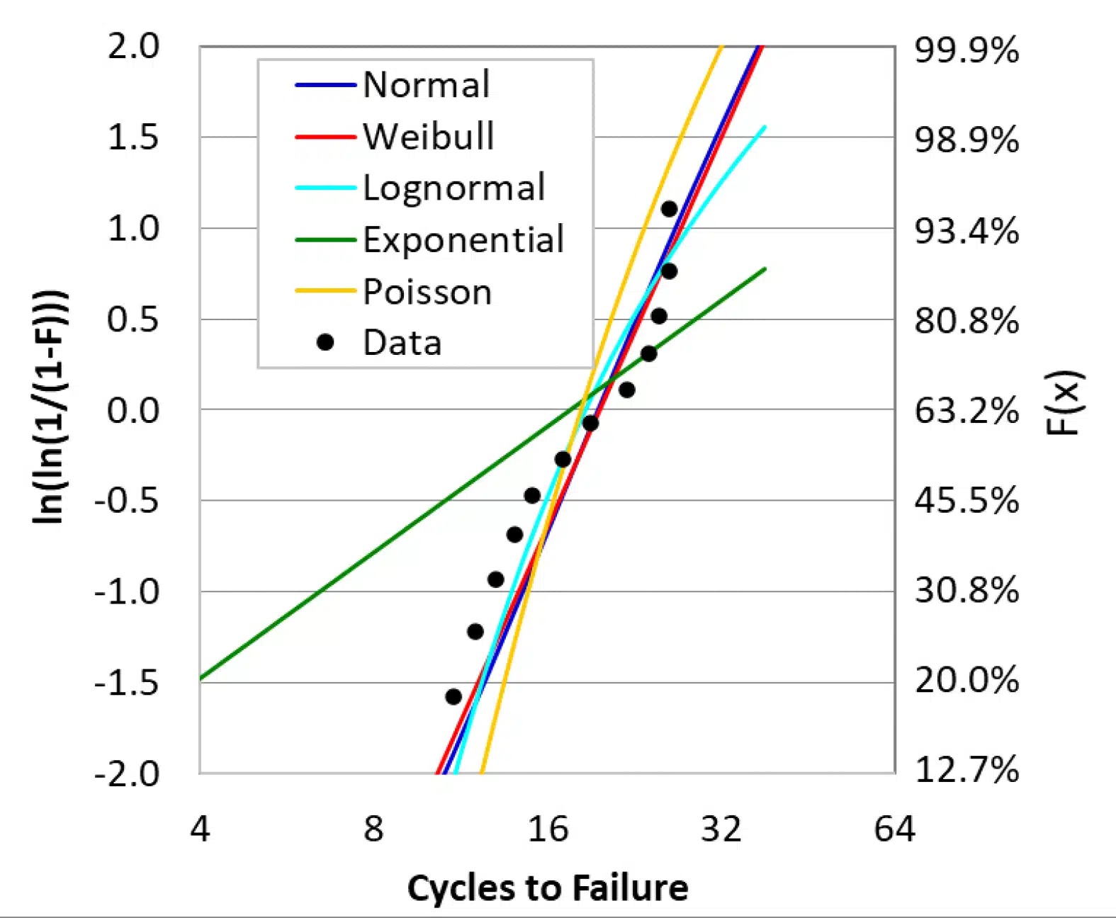
Readers who are familiar with Weibull plots will notice that Figure 2 and Figure 3 use an unusual format for showing Weibull fits. Traditionally, those plots use linearized axes so that the data are shown relative to a straight line. Figure 4 shows the data and the various distributions as plotted in this more conventional format.
Figure 4 Paper clip data from Figure 2, plotted on linearized axes
Conclusions
This article briefly discussed statistical distributions other than the normal distribution and specifically focused on the Weibull distribution. The analysis presented here showed that most, but not all, of the distributions provided a reasonably good fit when data for the entire population were available. However, the Weibull distribution was also able to directly determine an accurate representation of reliability data, even when testing had been stopped before all samples were tested.
Different distribution models are used for different types of analyses. It is important that, when using these different distributions, one has some understanding of why a given distribution is typically used and to recognize its limits.
References
1 Interested readers can find the Weibull probability distribution function from any number of sources. Since it is somewhat less intuitive than the cumulative distribution and not really relevant to the point being made in this article, I’m not including it here.
2 The syntax to use this function to determine the rank of a value of X within a set of data Y, use =rank(X,Y,1) where 1 specifies ascending order so that the first failure is 1, the second failure 2, etc.
3 The 3-parameter Weibull distribution includes an additional value, x0, which is offset value that forces the function to have a value of F(x0) = 0. The term x0, which corresponds to a failure-free life of the component, is physically useful but mathematically somewhat problematic since it prevents the Weibull distribution from being directly linearized.
- Ross Wilcoxon, “Statistics Corner – Probability”, Electronics Cooling Magazine, Spring 2020
- J. S. Milton and Jesse Arnold, Introduction to Probability and Statistics: Principles and Applications for Engineering and the Computing Sciences, McGraw-Hill, 1986, pp. 297-308
- Ross Wilcoxon, “Statistics Corner – Regression Analysis”, Electronics Cooling Magazine, Fall 2021

