ABSTRACT
Reliability verification often requires that a specific number of components be tested to a predetermined level of testing to demonstrate that none of the samples fail. This article describes a statistical approach for justifying the use of fewer samples by subjecting them to a more severe level of testing.
BACKGROUND
Reliability verification often includes accelerated testing in which a set of components must survive a prescribed set of severe environmental conditions. For example, components used in many avionics systems are commonly required to demonstrate solder joint integrity for 500 thermal cycles of -55 to +125°C [1]. One question that may arise in reliability testing is how many components must pass the test to demonstrate reliability. The number of components needed in a test is related to both the reliability that is to be demonstrated and the confidence level required for the results. Bayes (Success Run Theorem) formula13 provides a relationship between these three parameters [2] and can be written as shown in Equation {1}.
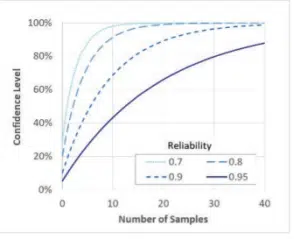
In this equation, R is the reliability, C is the confidence level and n = number of samples that are tested. Both the reliability and the confidence level have values between 0 and 1. Figure (1) plots the confidence level resulting from different samples sizes for select values of reliability, as a function of the number of samples. Equation {1} can be rearranged to show the number of samples required for a given reliability and confidence level, as shown in Equation {2}.
Figure 1. Reliability and confidence level for different sample sizes.
To demonstrate, for example, a reliability of 90% with a confidence level of 80%, a test would need to include at least 15 components14.
ANALYSIS
Established test procedures often define how many components must be included in a given test, presumably based on an assessment of the reliability and confidence level required. In some cases, there may be a desire to test a different number of components than what has been prescribed for a test. This may occur if the components are extremely expensive or if the evaluation approach, which determines whether a component has failed, is very expensive or time consuming.
Reducing the number of samples in a reliability test reduces the confidence level that a given test demonstrates a particular reliability value. However, this can be offset by testing components more severely (to demonstrate a higher reliability) and thereby justify the use of a smaller number of test samples. This article describes a statistical analysis that provides a basis for adjusting the severity of testing to reduce the number of test components required to demonstrate the same reliability and confidence level as a larger population. This analysis has been described by many others, such as in [2].
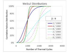
The analysis is based on the assumption that the failure distribution of the test articles follows a Weibull distribution. As described previously, the Weibull distribution provides a relationship between the number of test cycles and the population’s failure rate. The Weibull distribution is often used to analyze failure data and can be defined as shown in Equation {3}.
Figure 2. Weibull distributions
Regardless of the shape factor, all distributions with the same characteristic life cross through that value at 63.2%, hence the characteristic life also being known as N63. The cumulative failure distribution begins at zero and as the number of cycles increases asymptotically approaches 100%. The transition from F = 0 to F = 1 is sharper when the shape factor is larger. In terms of the more familiar Normal distribution, the characteristic life is analogous to the median of the population while the shape factor is analogous to the inverse of the standard deviation.
The failure distribution is related to the reliability by:
In other words, if 5% of a population has failed it has a reliability of 95%.
Equations {1}, {3}, and {4} can be combined to determine the number of thermal cycles required to demonstrate the same confidence level for a given reliability level for the different sample sizes. Combining Equations {1} and {3} relates the Weibull coefficients to the reliability:
Combining this with Equation (4) produces a relationship between the confidence level and the Weibull coefficients, leading to Equation (6) after taking the natural log of both sides.
If components from the same population with a given characteristic life and shape factor are used in two tests with different sample sizes (n), Equation {6} can be written as:
 {7)
{7)
In this equation, n1 and n2 are the sample sizes in tests 1 and 2 respectively while N1 and N2 are the numbers of thermal cycles used in tests 1 and 2 respectively. The last two terms in Equation {7} can be rearranged to produce:
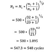
Equation {8} provides a method for calculating how many additional thermal cycles must be conducted for a test population with a reduced size. For example, consider a test that mandates that a population of 32 samples must survive for 500 thermal cycles. However, only 20 samples are available for testing. Assuming that the population will exhibit a failure distribution with a Weibull shape factor of 5, the number of thermal cycles required would be:
The required number of cycles is rounded up to the nearest whole number.
The critical assumption in determining an equivalent number of thermal cycles for a test is the value used for the Weibull shape factor. The shape factor depends on the type of component being tested, the type of test, and the consistency of the manufacturing build. One study, for example, has found that thermal cycle testing of surface mount components on assemblies built in a production environment had shape factors in the range of 3-6 [3]. This range seems reasonable based on this author’s experience, but it can vary depending on the consistency of the manufacturing processes as well as the type of component.
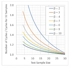
For reference, Figure (3) plots equation {8} for a number of values of shape factors and assuming a standard test population size of 32 components. For example, consider a standard test that requires that 32 components survive 100 cycles. If the component is assumed to have a shape factor of 3, and is tested with only 10 samples, the test would need be conducted for ~1.45x (145) cycles to demonstrate the same confidence level.
Figure 3. Equivalent test cycles for reduced sample size
One should be cautious in applying this approach to justify substantially reducing the number of samples by testing more severely. For example, with this approach one could theoretically reduce the sample size for a test population with shape factor of 3 from 32 to 3 by doubling the test duration. This is dangerous due to the risk of initiating a new failure mechanism that would not otherwise appear in a shorter accelerated test. In addition, the uncertainty of the shape factor for a given population is magnified when used with larger ratio of test cycles as shown in Equation (8). As a rule of thumb, one should generally not apply Equation (8) to justify a smaller sample size that requires increasing the test duration by more than ~40%.
SUMMARY
This article described an approach for determining how many additional thermal cycles are required to meet a given reliability level if testing is conducted with fewer than the standard number of test samples. The approach assumes that the failure distribution of the components follows a Weibull distribution of cumulative failure as a function of test cycles. It also assumes that the minimum expected Weibull shape factor for the component populations can be estimated with a reasonable degree of confidence.
References
13This equation is based on setting the cumulative distribution function for a binomial distribution to be equal to 1 minus the confidence level.
14Equation {2} finds the number of samples to be n = 14.27, which is rounded up to 15.
1. Hillman, et al., “The Impact of Reflowing a Pbfree Solder Alloy using a Tin/Lead Solder Alloy Reflow Profile on Solder Joint Integrity”, Int. Conf. on Lead-free Soldering, CMAP 2005, Toronto
2. Lipson and Sheth, “Statistical Design and Analysis of Engineering Experiments”, McGraw-Hill, 1973
3. Liu and Lewis, “A Comparison of Statistical Distribution Functions to Predict BGA Attach Reliability”, IEEE Transactions on Components and Packaging Technologies, Vol. 31, Issue. 3, 2008

 {7)
{7)