INTRODUCTION
After a couple of decades in the industry, I have observed that a number of experienced engineers can be intimidated by the topic of statistics—these columns will attempt to reduce the level of intimidation. While I have been interested in statistics for a few decades now, I don’t claim to be an expert. I will do my best to get things as right as I can, as well as to make things useful and practical.
Statistical analysis is needed because data will always have some degree of uncertainty; a value that we determine from a single measurement, or even a set of measurements, is not necessarily going to tell us exactly what value we will determine with additional measurements. Statistical analysis uses the mathematics of probability to create tools that we can use to deal with that uncertainty. This column discusses some aspects of probability concepts to set the basis for how the mathematics of probability can be applied to address uncertainty in statistical analysis.
Any discussion of statistical analysis must include a discussion on probability. Since the entire field of probability and statistical analysis began with gamblers attempting to improve their chances of winning, it seems appropriate that this discussion on probability begins with a game of chance: namely, throwing dice.
To begin, I assume that we have an infinite amount of time and patience that allows us to make a lot of throws, the dice that are not loaded (on any given throw they are equally likely to fall with any of its sides up), and we are not playing Dungeons & Dragons, so our dice only have six sides. In other words, I will use an Excel spreadsheet to simulate throwing dice. I trust that the random function is, in fact, fairly random, and that I can calculate the result of throwing a die with the equation “=ROUNDDOWN(RAND()*6,0)+1”.
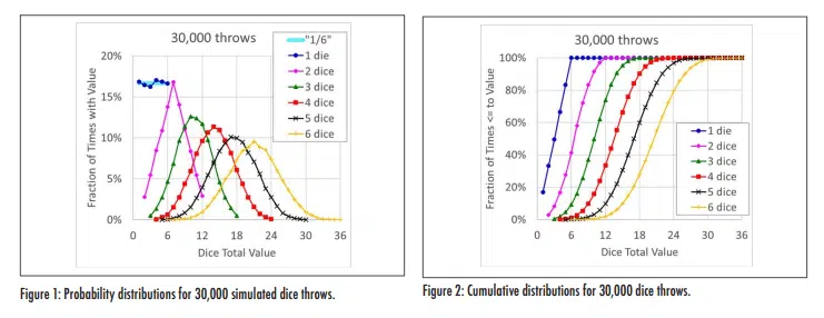
Figure 1 shows what fraction of 30,000 throws of 1-6 dice, as calculated using a simple Excel spreadsheet, had a total value of one to 36. For a single die, we would expect that the values one through six would each occur approximately 1/6th of the time— which is about what reasonably close to what was found in the calculations. As the number of dice included in the throws increases from one to six, the distributions change from a flat line to a triangle to an increasingly ‘bell shaped curve’.
Figure 2 shows the same data, but plots the cumulative distributions that show what portion of the throws had a total value that was equal to or less than a value between one and 36. One of the fundamental tenets of probability theory is that the probability of the sum of all possible outcomes is equal to one, which is both logical and illustrated in the figure. In these cumulative distributions, the plots transition from a straight line to a ‘tilted S shaped curve’ as the number of dice increases from one to six.
Readers with some (any?) background in statistics likely can see where this is going—the ‘bell’ and ‘tilted S’ shaped curves start to look like the normal distribution that is widely used in statistical analysis. The discussion on that topic will be in the next column in this series.
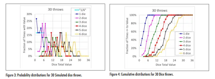
A question that may be asked is “What would happen if we had to use actual dice and we didn’t have the time needed to throw them 30,000 times?” Again, we can simulate that, with results shown for the probability and cumulative distributions for sets of only 30 throws of one through six dice in Figure 3 and Figure 4. Figure 3 is best described as an incoherent mess: for the ‘one die’ data, two values fell exactly on their expected theoretical value of 16.7%, while two other values were ~60% higher or lower than that. Data for more than one die do not appear to be much better behaved.
While the cumulative data for 30 throws, Figure 4, shows considerably more jitter than their counterparts for 30,000 throws (Figure 2), the cumulative distributions appear to be much less random than the raw distribution data (Figure 3). A comparison of Figure 3 and the curves that show the same data in Figure 4 illustrates why some data, such as from reliability testing, is often plotted in terms of a cumulative distribution rather than probability.
If a situation is governed by known physics, it can be relatively straightforward to estimate probabilities of a single event. In the case of rolling a single, non-loaded, six-sided die, it should seem obvious that there is a 1/6th chance of any of the six possible outcomes occurring. However, probability calculations can start to become less intuitive when we begin to consider combinations of multiple events. For example, consider the classic question that is considered to have been the beginning of mathematical analysis of probability—the likelihood of rolling a specific value within a specific number of attempts [1]. De Mere, a gambler in the 1600s, tended to win more often than not when he bet that he would roll a six within four attempts. His reasoning for why he would win was that the chances of rolling a six in one roll was 1/6th, so in four rolls his chances should be 4 * 1/6 = 2/3. Since that value is larger than 50% and he was playing even odds (the loser pays the same amount regardless of who it is), he had concluded that it was, on average a winning bet. But when he extended the game to two dice and gave himself 24 attempts to roll a double six, which by his reasoning should have had the same probability (24 * 1/6 * 1/6 = 2/3), he began to lose money. He asked the mathematician Blaise Pascal to help him understand why his luck had changed.
When calculating probabilities of multiple events, two things that should be kept in mind are that the calculated probability of any outcome must never exceed 100%, and that it is often useful to think in terms of an event not happening. In de Mere’s case, one simply has to consider the first point to recognize that his equation was incorrect. If the chances of rolling a six in four attempts is 2/3, then that equation states that the probability of rolling a six in eight attempts will be 133% (4/3). Clearly, this is not possible. To correctly determine the probability of rolling a six in four attempts, one can consider the probability of not rolling a six in one attempt and multiply that times itself four times. The probability of not rolling a six is (5/6 = 83.3%), so the probability of not rolling a six in four attempts is (5/6)4 = 48.2%. Since the probability of not rolling a six in those four attempts plus the probability of rolling a six in the same attempts must equal 100%, the probability of rolling a six in four attempts is 100%-48.2% = 51.8%. This probability is greater than 50%, so with even odds it makes sense that de Mere was coming out ahead. On the other hand, when using the same approach the probability of rolling double sixes in 24 attempts can be calculated as 1 – (35/36)24 = 49.1%, which is less than 50% and therefore not a good bet at even odds.
SUMMARY
Probability theory is fascinating and, even the most cursory overview of it, encompasses far more than can be addressed in this short article. This is particularly true if one considers the topic of conditional probability [2], in which the probability of an event depends on another probabilistic event. The example described in this article illustrates that, in a reasonably well-behaved population of data, the effects of measurement variability tend to wash out and lead us to familiar-looking distributions. But it may require a lot of samples from that population to get there. If we only look at a small portion of the population, the distribution won’t necessarily appear as a nice bell shape.
Future articles in this series will discuss some of the statistical approaches used to extract useful information and understand the distribution characteristics of data sets that are smaller than 30,000 that led to the smooth curves shown in Figures 1 and 2. Topics will include different parameters used to characterize a data set, what confidence we have regarding the uncertainty of those parameters, different models for distributions and how to use them, how to determine if one set of data is different from another, how many samples do we need for a given test, etc.
REFERENCES
1. https://introductorystats.wordpress.com/2010/11/12/onegambling-problem-that-launched-modern-probabilitytheory/, accessed August 24, 2019
2. https://www.probabilitycourse.com/chapter1/1_4_0_ conditional_probability.php


