Modeling Multiple Heat Source Problems In Electronic Systems

Introduction

Readers of ElectronicsCooling know about the rapid pace of technological developments towards an increasingly higher level of miniaturization and, hence, an incredible increase of dissipation power densities. Thus, restating some very well known facts (such as, we have already attained a level of power density that is comparable to nuclear power stations) would not be of much use.

In fact, what we are experiencing is a new era in thermal management challenges that is due to a qualitative change in the problem nature, in addition to the quantitative character. The keyword to pinpoint is multiplicity. Chip Multi�core Processors (CMP), Multi Chip Modules (MCM), 3D technology, Stacked Dies � are all technologies where the word multiple appears either explicitly or implicitly. Regardless of the particular technology or the length scale involved, a thermal management engineer mainly sees a multiple heat source object. Each heat source may be activated independently. Temperature gradient values and even directions (hence heat flow direction), maximum temperature point (or even zone) may all change depending on loading conditions.

In the following discussion, both convection and conduction heat transfer modes will be systematically compared. Both common and different features are instructive. Only steady state problems will be addressed for simplicity, although the discussion is also valid for dynamic problems [1].

The reason why this may pose a real modeling challenge to the thermal management engineer, for heat transfer by convection, lies deeply in classical scholar heat transfer textbooks. To be honest, circuit theory classical textbooks are not quite innocent either! In fact, the traditional way of modeling convection heat transfer uses heat transfer coefficient h:

Q₁₂ = h A (T₁ � T₂) (1)

relating the heat Q₁₂ flowing from point 1 to point 2 with temperatures at these points T₁ and T₂, the heat transfer area A and h. For heat transfer by conduction, there is a parallel to Equation (1), using the junction to case thermal resistance Θ_jc:

Q_jc = (1/Θ_jc) (T_j � T_c) (2)

where T_j and T_c refer to junction and case temperatures respectively. The parallel between hA and 1/Θ_jc is evident.

Seeing heat transfer as a phenomenon between two points bears two fundamental problems, which will shortly be discussed due to the difference between real life 3D problems and simple 1D problems. The latter are mainly encountered in textbooks rather than in real life.

Problem 1: We Only Have Two Points

For convection problems, in order to obtain the ‘magic number’ h, the heat transfer coefficient, intended to model heat transfer from a (single) heat source to a (single) heat sink, we usually conduct many experiments for an endless set of geometries. Thousands of correlations proliferate in textbooks. Would it be astonishing that none of these correlations treat the case of two or more heat sources? Of course not, because even if we were able to produce the tremendous set of correlations for all possible combinations, how could we use the result in an equation like (1) having only one heat source and one heat sink temperature.

The solution of such a problem has been proposed by Moffat, with his adiabatic heat transfer coefficient [2] concept. The idea is simple, like all brilliant ones. In fact, heat transfer by forced convection, for a given fluid flow field, is linear in terms of temperature and heat flux fields. Hence, one may address the above problem using the principle of superposition as follows:

• All existing heat sources or sinks are grouped in one set numbered from 1 to N
• Source number 1 (the junction, for example) is always activated, in addition to source i; all other sources are kept adiabatic. By repeating this experiment with different sources or sinks (i=2 to N) we get:

 

where Q_i is the heat out of source/sink i, and M_ij is in general a non�symmetric matrix. We still need to obtain a large number (in fact a whole matrix) of coefficients, but at least we know now how to use them!

For conduction problems, it has long been recognized that, although heat dissipated from a (single) heat source (the junction at T_j) will ultimately reach ambient (at T_a), heat paths may be different depending on how a dissipating object is cooled. To understand this, take for instance a package in a system (the same could be said of a transistor in a chip or a computer in a data center). The inside of the package has different thermal resistances from the hotspot(s) to top, bottom or sides. This is an intrinsic feature that does not depend on how the package is used.

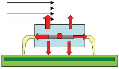
Figure 1. Outside boundary conditions (cooling fluid properties, velocity and temperature, PCB composition �) influence internal heat flow paths.

However, package cooling at different faces largely depends on outside conditions. To address this issue, we cannot just split the junction-to-ambient resistance Θ_ja into two independent resistances: a junction-to-case + a case-to-ambient resistance. In fact, the heat flow distribution inside the package to outer faces will vary depending on outside boundary conditions. Consider Figure 1. When the flow comes from the left side, the left side heat flux leaving the package will be larger than the right side heat flux. Hence, it would be impossible to obtain a single Boundary Condition Independent (BCI) ‘equivalent’ junction-to-case thermal resistance. Even with only one internal heat source, the package as a whole should be viewed as a multiple heat sink object, corresponding to different dissipation paths. This closely resembles the multiple heat source issue. Hence, it is imperative to model it with a ‘matrix’ like representation (analogous to M_ij).

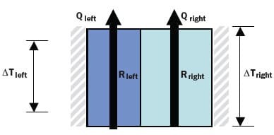
Figure 2. A simple illustrative example of profile effect.

One of the major contributions in this respect is the BCI concept, see [3] as well as the first BCI compact models developed by the Delphi team. It was formulated in the form of a resistive network, but it is a simple algebraic exercise to transform the resistive network into a matrix as in eq. 3. In this case the matrix is symmetric. Obtaining matrix elements (or resistive networks) can be done in many different ways, see [1] for an overview.

Any linear problem, with multiple inputs/outputs can be modeled by a matrix of coefficients relating them, but not any matrix can be a suitable candidate to model real physics. In a general approach, based on thermodynamics fundamentals, mathematical conditions to be satisfied by this matrix were obtained [4], both for conduction and convection, giving the first basis for a unified theory of compact thermal models. Note that for the convection case, the matrix has to be non-symmetric, the reason being the directional dependence of the flow. Hence, it is impossible to represent it in the form of resistors or capacitors.

Problem 2: We Shouldn’t Have Worked With “Points” Anyway!

The second mandatory issue for multiple heat sources is that of temperature profiles. Heat exchange is not done between points but between surfaces with a certain profile representing the flux distribution. This is in fact also present for single heat source problems, but it is easy to get rid of it because of the similarity of profiles in different situations.

To prove this without doing a lot of math, let us consider an object composed of two boxes, both with insulated sidewalls and both exchanging heat with the surroundings at top and bottom surfaces only. Because sidewalls are insulated, each object can be viewed as a simple 1D thermal resistor having the well-known value: d/kA where d is the thickness, k the thermal conductivity and A the cross-sectional area. Suppose either d or k were different, which would produce two different resistors in parallel, one on the left R_left, the other on the right R_right. If we impose, for example, a non-uniform profile on the top face, e.g., the left part takes a portion of Q_tot, the right the remainder part (1 � ) of Q_tot. Then:

The extremely simple equation (4), in which profile shape is represented by a single parameter , tells us a lot about compact thermal models!

• The exact shape of the heat flux profile influences the total thermal resistance.
• In case the object was uniform in thickness and material, R_left = R_right and hence R_tot becomes independent of , i.e., independent of the profile. Now, do you believe that in engineering practice there are many objects that are perfectly homogeneous in thickness and in physical properties? If you say yes, than you can claim that profile is immaterial and that we can always extract an “equivalent” thermal resistance that models thermal behavior with any profile! If you say no, than you have to admit the inevitable fact: Profile is crucial in extracting a compact thermal model.
• Suppose the object was not uniform, R_left ≠ R_right, but the profile is fixed (i.e., values may change, but not the shape). As a result, R_tot will be fixed. In this case, R_tot will correctly model a whole set of problems restricted by the fact that the profile is fixed. That is precisely what happened for single heat source problems: changing boundary conditions within practical ranges would not dramatically change the profile, at least not qualitatively. With a good optimization technique and intelligently selected practical test cases [3], one could successfully get an optimum thermal model that models all real life situations with the smallest possible error. However, can we say the same with multiple independent heat sources? Unfortunately not, because the shape of the profile may drastically change, as is obvious when we consider two sources for the three combinations on-off, off-on and on-on. A discussion of the effect of profile on compact model errors is available [4].

 

A Plausible Solution: The Flexible Profile Technology

To overcome above mentioned problems the flexible profile technology was developed [5]. On each node (i.e., on each zone of heat exchange with the surroundings) of the object to be modeled, it is possible to describe profiles (of both heat flux and temperature) by a truncated series. Practically speaking, a constant, a straight line and a parabola can be combined to represent sufficiently well the majority of real life profiles. However, nothing prevents us from having more terms in the series if necessary. In fact, if the number of terms increases, we quickly approach the exact solution of the heat transfer problem.

Instead of studying the compact model for a given rigid profile, or set of profiles (which is the case for most of classical approaches), the flexible profile technology studies the object response to each component in the series independently. For example the effect of a uniform heat flux on node 1 is studied first, followed by the effect of one that varies linearly etc. The same is repeated for all other nodes. By combining all results in a suitable matrix, we can quickly see the effect of each heat flux component of the series at each node on any other heat flux or temperature component at any other node. In practice, matrix components are not really obtained individually, but by blocks. Thus, any arbitrarily applied heat flux (or temperature) profile can be treated (hence the name: flexible profile) by decomposing it onto the truncated series, obtain the response to each individual component and finally sum the results to get the response to that arbitrary applied profile.

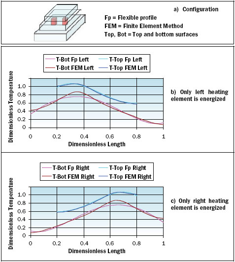
Figure 3. Temperature profiles through the source centers for a package with
two heating sources using flexible profile technology.

Results are astonishingly good, including in particular the multiple heat source case, as can be seen from Figure 3 showing a temperature plot through the centers of the sources from left to right. The case treated does not correspond to a particular package, but was selected to exhibit all possibilities offered by the technology, in particular non-uniform lateral dimension, lateral surface heating, different thermal conductivities and different types of boundary conditions. It is a pyramidal structure where heat may be generated by either of the two cubic heaters in the middle block.

Boundary conditions are as follows:

• Ambient temperature = 20�C
• Boundary conditions on side, top and bottom surfaces have different types and values.
• A volumetric heating rate of 12.5 MW/m³ can be generated in either of the two heating elements.

 

Another important advantage of the flexible profile technology is that it does not only give the temperature at a node, but also its tangential gradient. This information that is inaccessible in classical approaches is of paramount importance to estimate thermally induced stresses and hence assess object reliability.

In short �

If you want to model modern multiple heat source problems, you should consider models with multiple nodes and multiple modes on each node.

References

1. Sabry, M.N., “Dynamic Compact Thermal Models Used for Electronic Design: a Review of Recent Progress,” Proceedings of IPACK03, Maui, Hawaii, USA, Interpack, 2003-35185.
2. Moffat, R., “The Benefits Of Using Hadiabatic in Thinking about Electronics Cooling,” ElectronicsCooling Vol.10, No.1, 2004.
3. Lasance, C, Den Hertog, D. and Stehouwer, P., “Creation and Evaluation of Compact Models for Thermal Characterization Using Dedicated Optimization Software”, 15th Annual IEEE Semiconductor Thermal Measurement and Management Symposium, SEMI-THERM, 1999, p.1.
4. Sabry, M.N., “Compact Thermal Models for Electronic Systems,” IEEE � CPT, Part A, Vol. 26, 2002, pp. 179-185.
5. Sabry, M.N., “Compact Thermal Models: A Global Approach,” 1st International Conference on Thermal Issues in Emerging Technologies, Theory and Applications, ThETA1, Cairo, Egypt, 2007.